Page 33 - Read Online

Hansen et al. Microstructures 2023;3:2023029 https://dx.doi.org/10.20517/microstructures.2023.17 Page 11 of 17

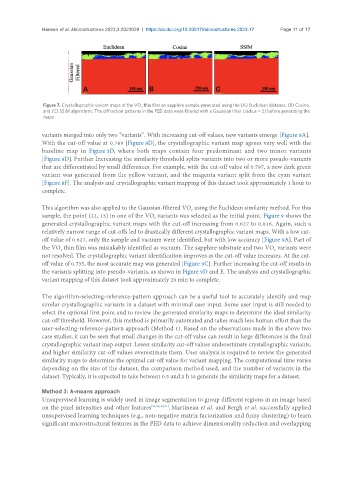
Figure 7. Crystallographic variant maps of the VO thin film on sapphire sample generated using the (A) Euclidean distance, (B) Cosine,
2
and (C) SSIM algorithms. The diffraction patterns in the PED data were filtered with a Gaussian filter (radius = 5) before generating the
maps.

variants merged into only two “variants”. With increasing cut-off values, new variants emerge [Figure 8A].
With the cut-off value at 0.769 [Figure 8D], the crystallographic variant map agrees very well with the
baseline map in Figure 3D, where both maps contain four predominant and two minor variants
[Figure 8D]. Further Increasing the similarity threshold splits variants into two or more pseudo-variants
that are differentiated by small differences. For example, with the cut-off value of 0.787, a new dark green
variant was generated from the yellow variant, and the magenta variant split from the cyan variant
[Figure 8F]. The analysis and crystallographic variant mapping of this dataset took approximately 1 hour to
complete.

This algorithm was also applied to the Gaussian-filtered VO using the Euclidean similarity method. For this
2
sample, the point (22, 13) in one of the VO variants was selected as the initial point. Figure 9 shows the
2
generated crystallographic variant maps with the cut-off increasing from 0.627 to 0.816. Again, such a
relatively narrow range of cut-offs led to drastically different crystallographic variant maps. With a low cut-
off value of 0.627, only the sample and vacuum were identified, but with low accuracy [Figure 9A]. Part of
the VO thin film was mistakably identified as vacuum. The sapphire substrate and two VO variants were
2
2
not resolved. The crystallographic variant identification improves as the cut-off value increases. At the cut-
off value of 0.735, the most accurate map was generated [Figure 9C]. Further increasing the cut-off results in
the variants splitting into pseudo-variants, as shown in Figure 9D and E. The analysis and crystallographic
variant mapping of this dataset took approximately 20 min to complete.

The algorithm-selecting-reference-pattern approach can be a useful tool to accurately identify and map
similar crystallographic variants in a dataset with minimal user input. Some user input is still needed to
select the optional first point and to review the generated similarity maps to determine the ideal similarity
cut-off threshold. However, this method is primarily automated and takes much less human effort than the
user-selecting-reference-pattern approach (Method 1). Based on the observations made in the above two
case studies, it can be seen that small changes in the cut-off value can result in large differences in the final
crystallographic variant map output. Lower similarity cut-off values underestimate crystallographic variants,
and higher similarity cut-off values overestimate them. User analysis is required to review the generated
similarity maps to determine the optimal cut-off value for variant mapping. The computational time varies
depending on the size of the dataset, the comparison method used, and the number of variants in the
dataset. Typically, it is expected to take between 0.5 and 2 h to generate the similarity maps for a dataset.

Method 3: k-means approach
Unsupervised learning is widely used in image segmentation to group different regions in an image based
on the pixel intensities and other features [21,22,40,41] . Martineau et al. and Bergh et al. successfully applied
unsupervised learning techniques (e.g., non-negative matrix factorization and fuzzy clustering) to learn
significant microstructural features in the PED data to achieve dimensionality reduction and overlapping