Page 36 - Read Online

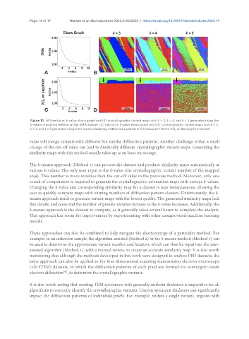
Page 14 of 17 Hansen et al. Microstructures 2023;3:2023029 https://dx.doi.org/10.20517/microstructures.2023.17

Figure 10. (A) Inertia vs. k-value elbow graph and (B) crystallographic variant maps with k = 3, k = 4, and k = 5 generated using the
k-means clustering method on the SMA dataset. (C) Inertia vs. k-value elbow graph and (D) crystallographic variant maps with k = 3,
k = 4, and k = 5 generated using the k-means clustering method on a portion of the Gaussian-filtered VO on the sapphire dataset.
2
value will merge variants with different but similar diffraction patterns. Another challenge is that a small
change of the cut-off value can lead to drastically different crystallographic variant maps. Generating the
similarity maps with this method usually takes up to an hour on average.

The k-means approach (Method 3) can process the dataset and produce similarity maps automatically at
various k-values. The only user input is the k-value (the crystallographic variant number of the mapped
area). This number is more intuitive than the cut-off value in the previous method. Moreover, only one
round of computation is required to generate the crystallographic orientation maps with various k-values.
Changing the k-value and corresponding similarity map for a dataset is near instantaneous, allowing the
user to quickly compare maps with varying numbers of diffraction pattern clusters. Unfortunately, the k-
means approach tends to generate variant maps with the lowest quality. The generated similarity maps lack
fine details, and noise and the number of pseudo-variants increase as the k-value increases. Additionally, the
k-means approach is the slowest to compute, as it generally takes several hours to complete the analysis.
This approach has room for improvement by experimenting with other unsupervised machine learning
models.

These approaches can also be combined to help mitigate the shortcomings of a particular method. For
example, in an unknown sample, the algorithm-assisted (Method 2) or the k-means method (Method 3) can
be used to determine the approximate variant number and location, which can then be input into the user-
assisted algorithm (Method 1), with a manual review, to create an accurate similarity map. It is also worth
mentioning that although the methods developed in this work were designed to analyze PED datasets, the
same approach can also be applied to the four-dimensional scanning transmission electron microscopy
(4D-STEM) datasets, in which the diffraction patterns of each pixel are formed via convergent-beam
electron diffraction , to determine the crystallographic variants.
[43]

It is also worth noting that creating TEM specimens with generally uniform thickness is imperative for all
algorithms to correctly identify the crystallographic variants. Uneven specimen thickness can significantly
impact the diffraction patterns of individual pixels. For example, within a single variant, regions with