Page 28 - Read Online

Page 6 of 17 Hansen et al. Microstructures 2023;3:2023029 https://dx.doi.org/10.20517/microstructures.2023.17

each pixel will be compared to all reference patterns, and the one with the highest similarity value will be
used for the variant assignment of pixels. Each variant is represented by a color in the map. Before going
into the detailed mapping results using the first method, we will briefly discuss similarity quantification
using Euclidian distance, Cosine, and SSIM algorithms.

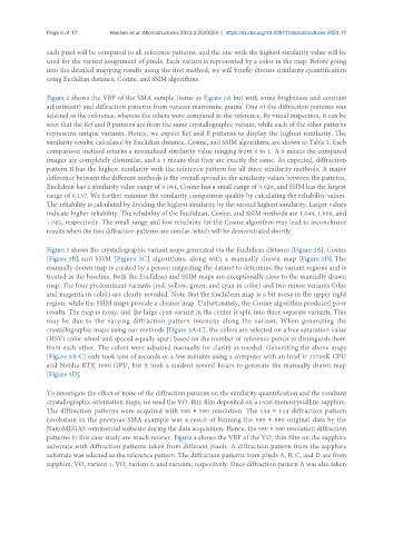
Figure 2 shows the VBF of the SMA sample (same as Figure 1A but with some brightness and contrast
adjustment) and diffraction patterns from various martensite grains. One of the diffraction patterns was
selected as the reference, whereas the others were compared to the reference. By visual inspection, it can be
seen that the Ref and B patterns are from the same crystallographic variant, while each of the other patterns
represents unique variants. Hence, we expect Ref and B patterns to display the highest similarity. The
similarity results, calculated by Euclidian distance, Cosine, and SSIM algorithms, are shown in Table 1. Each
comparison method returns a normalized similarity value ranging from 0 to 1. A 0 means the compared
images are completely dissimilar, and a 1 means that they are exactly the same. As expected, diffraction
pattern B has the highest similarity with the reference pattern for all three similarity methods. A major
difference between the different methods is the overall spread in the similarity values between the patterns.
Euclidean has a similarity value range of 0.081, Cosine has a small range of 0.026, and SSIM has the largest
range of 0.137. We further examine the similarity comparison quality by calculating the reliability values.
The reliability is calculated by dividing the highest similarity by the second highest similarity. Larger values
indicate higher reliability. The reliability of the Euclidean, Cosine, and SSIM methods are 1.044, 1.006, and
1.083, respectively. The small range and low reliability for the Cosine algorithm may lead to inconclusive
results when the two diffraction patterns are similar, which will be demonstrated shortly.

Figure 3 shows the crystallographic variant maps generated via the Euclidean distance [Figure 3A], Cosine
[Figure 3B], and SSIM [Figure 3C] algorithms, along with a manually drawn map [Figure 3D]. The
manually drawn map is created by a person inspecting the dataset to determine the variant regions and is
treated as the baseline. Both the Euclidean and SSIM maps are exceptionally close to the manually drawn
map. The four predominant variants (red, yellow, green, and cyan in color) and two minor variants (blue
and magenta in color) are clearly revealed. Note that the Euclidean map is a bit noisy in the upper right
region, while the SSIM maps provide a cleaner map. Unfortunately, the Cosine algorithm produced poor
results. The map is noisy, and the large cyan variant in the center is split into three separate variants. This
may be due to the varying diffraction pattern intensity along the variant. When generating the
crystallographic maps using our methods [Figure 3A-C], the colors are selected on a hue saturation value
(HSV) color wheel and spaced equally apart based on the number of reference points to distinguish them
from each other. The colors were adjusted manually for clarity as needed. Generating the above maps
[Figure 3A-C] only took tens of seconds or a few minutes using a computer with an Intel i7 13700K CPU
and Nvidia RTX 3080 GPU, but it took a student several hours to generate the manually drawn map
[Figure 3D].

To investigate the effect of noise of the diffraction patterns on the similarity quantification and the resultant
crystallographic orientation maps, we used the VO thin film deposited on a c-cut monocrystalline sapphire.
2
The diffraction patterns were acquired with 580 × 580 resolution. The 144 × 144 diffraction pattern
resolution in the previous SMA example was a result of binning the 580 × 580 original data by the
NanoMEGAS commercial software during the data acquisition. Hence, the 580 × 580 resolution diffraction
patterns in this case study are much noisier. Figure 4 shows the VBF of the VO thin film on the sapphire
2
substrate with diffraction patterns taken from different pixels. A diffraction pattern from the sapphire
substrate was selected as the reference pattern. The diffraction patterns from pixels A, B, C, and D are from
sapphire, VO variant 1, VO variant 2, and vacuum, respectively. Since diffraction pattern A was also taken
2
2