Page 120 - Read Online

Page 6 of 19 Peng et al. Soft Sci. 2025, 5, 38 https://dx.doi.org/10.20517/ss.2025.31

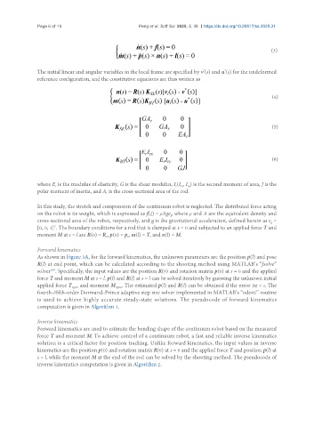
(3)

*
*
The initial linear and angular variables in the local frame are specified by v (s) and u (s) for the undeformed
reference configuration, and the constitutive equations are thus written as

(4)

(5)

(6)

where E is the modulus of elasticity, G is the shear modulus, I (I , I ) is the second moment of area, J is the
ry
rx
r
r
polar moment of inertia, and A is the cross-sectional area of the rod.
r
In this study, the stretch and compression of the continuum robot is neglected. The distributed force acting
on the robot is its weight, which is expressed as f(ξ) = ρAge , where ρ and A are the equivalent density and
g
cross-sectional area of the robot, respectively, and g is the gravitational acceleration, defined herein as e =
g
[0, 0, 1] . The boundary conditions for a rod that is clamped at s = 0 and subjected to an applied force T and
T
moment M at s = l are R(0) = R , p(0) = p , m(l) = T, and n(l) = M.
0
0
Forward kinematics
As shown in Figure 3A, for the forward kinematics, the unknown parameters are the position p(l) and pose
R(l) at end point, which can be calculated according to the shooting method using MATLAB’s “fsolve”
solver . Specifically, the input values are the position R(0) and rotation matrix p(0) at s = 0 and the applied
[28]
force T and moment M at s = l. p(l) and R(l) at s = l can be solved iteratively by guessing the unknown initial
applied force T and moment M . The estimated p(l) and R(l) can be obtained if the error Δe < ε. The
0guss
0guss
fourth-/fifth-order Dormand–Prince adaptive step size solver implemented in MATLAB’s “ode45’’ routine
is used to achieve highly accurate steady-state solutions. The pseudocode of forward kinematics
computation is given in Algorithm 1.

Inverse kinematics
Forward kinematics are used to estimate the bending shape of the continuum robot based on the measured
force T and moment M. To achieve control of a continuum robot, a fast and reliable inverse kinematics
solution is a critical factor for position tracking. Unlike forward kinematics, the input values in inverse
kinematics are the position p(0) and rotation matrix R(0) at s = 0 and the applied force T and position p(l) at
s = l, while the moment M at the end of the rod can be solved by the shooting method. The pseudocode of
inverse kinematics computation is given in Algorithm 2.