Page 75 - Read Online

Page 8 of 17 Cheng et al. J. Mater. Inf. 2025, 5, 53 https://dx.doi.org/10.20517/jmi.2025.61

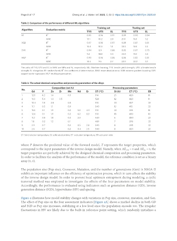
Table 2. Comparison of the performance of different ML algorithms
Training set Testing set
Algorithm Evaluation metric
TYS UTS EL TYS UTS EL
RF R 2 0.95 0.96 0.91 0.89 0.90 0.84
MAE 13.1 10.2 2.0 21.0 16.5 3.2
XGB R 2 0.97 0.96 0.97 0.89 0.87 0.81
MAE 10.4 10.3 1.2 22.3 18.5 3.3
2
SVR R 0.94 0.9 0.86 0.85 0.87 0.75
MAE 9.2 14.0 3.0 23.0 18.3 3.4
2
MLP R 0.90 0.96 0.86 0.86 0.83 0.81
MAE 18.4 9.5 2.7 23.0 22.2 3.7
The units of TYS/UTS and EL in MAE are MPa and %, respectively. ML: Machine learning; TYS: tensile yield strength; UTS: ultimate tensile
2
strength; EL: elongation; RF: random forest; R : the coefficient of determination; MAE: mean absolute error; XGB: extreme gradient boosting; SVR:
support vector regression; MLP: multilayer perceptron.

Table 3. The actual chemical composition and processing parameters of the alloys
Composition (wt.%) Processing parameters
No.
Gd Y Zn Zr Mn Nd Er ST (°C) St (h) ET (°C) ER
1 12.3 6.2 1.4 0.3 514 21 420 15
2 11.0 5.4 1.0 0.5 520 12 420 11
3 10.4 7.8 2.8 0.8 514 30 437 22
4 11.1 0.5 1.1 0.9 540 12 415 22
5 15.5 0.1 1.9 0.2 5.0 4.0 510 22 395 14
6 12.4 0.1 1.9 0.3 6.2 0.3 510 18 450 10
7 11.2 0.8 1.8 0.3 2.0 540 5 400 22
8 1.8 0.2 1.2 0.1 489 7 390 22
9 2.9 0.7 0.2 0.5 2.8 540 8 390 22
10 2.6 0.7 0.2 0.4 2.5 540 8 420 22
ST: Solid solution temperature; St: solid solution time; ET: extrusion temperature; ER: extrusion ratio.

where P denotes the predicted value of the forward model, T represents the target properties, which
correspond to the input parameters of the inverse design model. Namely, when AE = 0 and AE = 0, the
UTS
EL
target properties are perfectly achieved by the designed chemical composition and processing parameters.
In order to facilitate the analysis of the performance of the model, the reference condition is set as a binary
array (0, 0).

The population size (Pop size), Crossover, Mutation, and the number of generations (Gen) in NSGA-II
exhibit an important influence on the efficiency of optimization process, which in turn affects the stability
of the inverse design model. In order to prevent local optimum entrapment during modeling, a cyclic
traversal method was employed to investigate the effects of the four parameters on model stability.
Accordingly, the performance is evaluated using indicators such as generation distance (GD), inverse
generation distance (IGD), hypervolume (HV) and spacing.

Figure 4 illustrates how model stability changes with variations in Pop size, crossover, mutation, and Gen.
The effect of Pop size on the four assessment indicators [Figure 4A] shows a marked decline in both GD
and IGD as Pop size increases, stabilizing at a low level once the population exceeds 300. The irregular
fluctuations in HV are likely due to the built-in reference point setting, which randomly initializes a