Page 16 - Read Online

Page 10 of 17 Schertzer et al. J. Mater. Inf. 2025, 5, 5 https://dx.doi.org/10.20517/jmi.2024.69

in interpolation within the chemical space defined by the training set, making it a valuable tool for
optimizing new combinations of known monomers for improved AEM performance.

The TS, which tested the model’s ability to predict properties of known chemistries at different
temperatures, further showcased the advantage of MT learning. Figure 7 shows how the MT model captures
the expected linear trend (Arrhenius behavior) of hydroxide conductivity slightly beyond the temperature
range captured by the training dataset for three different polymers. As shown by the gray vertical dashed
lines, the linear regime stretches from 275 to 400 K. This ability to predict across different temperature
conditions is crucial for understanding real-world AEM performance, as operational environments in fuel
cells can vary widely.

Based on the performance of the MT models across all splits, we anticipate that the final model -
incorporating all curated data - will exhibit strong interpolative capabilities but currently has limited
extrapolative behavior to new monomer chemistries due to the small dataset size. The superior performance
of the MT model in the challenging PS suggests that increasing the size and chemical diversity of the dataset
will enhance its ability to predict novel chemistries. Its robust interpolative performance in the composition
and TS provides confidence in predicting the properties of new candidate copolymers composed of known
monomers. As the dataset grows, we expect improvements in both extrapolation and interpolation, leading
to more accurate predictions for entirely novel AEM polymer chemistries. In future work, we plan to
expand our dataset to include poly(aryl piperidinium), polynorbornene, and other advanced chemistries
and extend from just neat thermoplastics to also incorporating thermosets, composites, and blends.

SHapley Additive exPlanations (SHAP) analysis was used to add an element of interpretability to the ML
models by identifying the most important input features. Figure 8 shows the top ten most impactful
chemical features from most important (top) to least important (bottom). From the SHAP analysis, we
identified temperature and IEC as having the major impact on the model output, along with certain
chemical motifs such as quaternary ammonium ions, backbone toluene, and side chain length. The effect of
these chemical motifs on AEM fuel cell performance should be explored in future works, with this analysis
aiding in the explainable design of AEM membranes. As quaternary ammonium cations were found to be
one of the most descriptive chemical features, their effect on the AEM performance needs to be thoroughly
investigated.

Promising candidates and design suggestions
Our candidate set addresses the gaps in the AEM literature over the past 20 years. By enumerating all
captured chemistries at various monomer ratios, we explore the full spectrum of synthesized and
characterized monomer combinations. This comprehensive approach enables us to identify polymers with
fine-tuned properties without compromising the synthetic feasibility.

Among the approximately 11 million candidates generated, 6.5 million did not contain fluorine. Of these,
478 candidates met all the property criteria: anion conductivity of ≥ 100 mS/cm, maximum WU of ≤ 35 wt%,
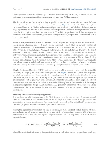
and maximum SR of ≤ 50 wt%. The expected improvement (EI) for each property for each candidate was
calculated using:

(4)

where δ for maximization is equal to the predicted mean at x, µ(x), minus the best-observed data point, f ,
best