Page 13 - Read Online

Schertzer et al. J. Mater. Inf. 2025, 5, 5 https://dx.doi.org/10.20517/jmi.2024.69 Page 7 of 17

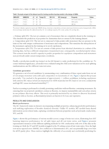
Table 1. Example snippet of the dataset used for training machine learning models in the design of AEMs
SMILES1 SMILES2 c1 c2 Temp (C) RH (%) IEC (meq/g) Property Value
-
Cc1cc(*)... (*)C(C... 37 63 25 100 2.33 OH Cond. (mS/cm) 12.1
Cc1cc(*)... (*)C(C... 37 63 25 100 2.33 WU (wt%) 17.4
Cc1cc(*)... (*)C(C... 37 63 25 100 2.33 SR (%) 7.2

The dataset includes copolymer repeat unit SMILES strings, monomer compositions, and associated experimental property measurements. AEMs:
Anion exchange membranes; RH: relative humidity; IEC: ion exchange capacity; WU: water uptake; SR: swelling ratio.

1. Polymer split (PS): The test set contains a set of monomers that are completely absent in the training set.
This simulates the prediction of properties for chemistries that are unseen by the training dataset.
2. Composition split (CS): The test set is composed of data points with monomers that are present in the
train set but with unique combinations of monomers and compositions. This simulates the interpolation of
the monomers captured in the training set to novel copolymers.
3. Temperature split (TS): The test set consists of data points from identical chemistries to a subset of the
training data, but has a different temperature measurement and, consequently, recorded property values.
This scenario tests the model’s capacity to predict properties for copolymer compositions and monomers
seen previously under unseen temperature conditions.

Finally, a production model was trained on the full dataset to make predictions for the candidate set. To
ensure statistical significance, all models were evaluated using five-fold cross-validation in five seed-splitting
randomizations and five different train-test ratios.

Candidate generation
We generate a set of novel candidates by enumerating every combination of three repeat units from our set
of 108 unique monomer units with each composition in increments of 10%. Figure 4 depicts this process
pictorially. This resulted in the generation of approximately 11 million candidates, including copolymers
with extreme IEC values (which are impractical for AEM materials; low IEC leads to low ionic conductivity
and high IEC causes mechanical instability) .
[3,8]
Further screening is performed to identify promising candidates without fluorine-containing monomers. By
ensuring that our proposed candidates contain no fluorine, we impose sustainability and cost as key criteria
in our polymer discovery efforts. This work is primarily motivated by our desire to discover functional
polymers with no fluorine, as fluorinated polymers are known to be toxic and expensive.

RESULTS AND DISCUSSION
Model performance
The MT framework trains on datasets encompassing multiple properties, enhancing predictive performance
and enabling exploration of broader chemical diversity. Unlike ST models, MT models learn shared
information across related tasks, capturing correlations between properties such as hydroxide conductivity,
WU, and SR.

Figure 5 shows the performance of various models across a range of train-test ratios, illustrating how MT
learning improves performance for all split types and all test-train ratios, and Figure 6 presents
representative instances of the different splitting methods for OH conductivity with 80% of the data in the
-
training set. Both the ST and MT models struggled in the PS setting across all test-train ratios. Note the high
root mean squared error (RMSE), low coefficient of determination (R ), and exceptionally large error bars
2
for all PS parity plots. These metrics highlight the difficulty of accurately and confidently predicting the