Page 85 - Read Online

Page 269 Liu et al. Intell Robot 2024;4(3):256-75 I http://dx.doi.org/10.20517/ir.2024.17

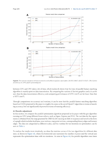
Figure 8. The runtime comparison of feature extraction with different graphics card models. (A) RTX 2080Ti; (B) GTX 1050Ti. CPU: Central
processing unit; GPU: graphic processing unit.

between GPU and CPU takes a lot of time, which indirectly shows that the time of parallel feature matching
algorithm is mainly spent on data transmission. By comparing the runtime of the two graphics cards, it can be
seen that the data transmission efficiency and computing performance of GTX 1050Ti are far lower than that
of RTX 2080Ti.

Through comparisons on accuracy and runtime, it can be seen that the parallel feature matching algorithm
based on CUDA proposed in the paper is roughly the same as the serial OpenCV algorithm in terms of match-
ing accuracy, but has significantly improved in terms of running efficiency.

4.2 Bundle adjustment
In this section, we compare the parallel optimization algorithm proposed in the paper with the g2o algorithm
running on CPU using different linear solvers, such as Eigen, Csparse and PCG. The test data for the experi-
ments is obtained from the map generated by ORB-SLAM running on Kitti 00 sequence and saved in the form
of a graph which includes keyframe-pose vertices, map point vertices, corresponding binary edges and ternary
edges. The data are categorized as different scales, and the runtime for ten iterations in optimization can be
seen in Table 3.

To analyze the results more intuitively, we draw the runtime curves of the two algorithms for different data
sizes, as shown in Figure 9A, where the horizontal axis represents the number of poses and the vertical axis
represents the optimization time with ten iterations. As seen in Figure 9A, the parallel algorithm runs faster