Page 80 - Read Online

Liu et al. Intell Robot 2024;4(3):256-75 I http://dx.doi.org/10.20517/ir.2024.17 Page 264

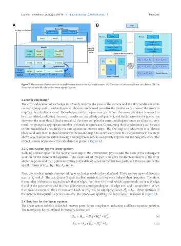
Figure 3. The process of error calculation and the construction for the linear system. (A) The chart of the parallel error calculation; (B) The
flow chart of parallel solution for linear system update.

3.2 Error calculation
The error calculation of each edge in BA only involves the pose of the camera and the 3D coordinates of its
connected map points, and independent threads can be used to realize the parallel calculation of the errors to
improve the calculation speed. Nevertheless, unlike the previous calculation, the errors calculated here need to
beaccumulated, indicatingthateachthreadisnotcompletelyindependent, andthedataneedstobeinteractive.
However, the more thread blocks are called, the more complex the corresponding resources are allocated. As a
result, assigning the appropriate number of threads is significant. Considering the shared memory can be used
within thread blocks, we divide the sum operation into two steps. The first step is to add errors in all thread
blocks and save them in shared memory; the second step is to sum the errors in the shared memory. The steps
above largely avoid the data interaction among thread blocks and greatly improve the running efficiency. The
overall process of parallel error calculation is given in Figure 3A.

3.3 Construction for the linear system
Building a linear system is the most critical step in the optimization process and the basis of the subsequent
solution for the incremental equation. The main task of this part is to solve the Jacobian matrix of the error
about the poses and map points according to the data obtained in the first two parts, and then determine the
specific forms of , , , and .

First, the Jacobian matrix corresponding to each edge needs to be calculated. There are two types of Jacobian
matrix: and . The calculation of each Jacobian matrix is a completely independent operation. Therefore,
the number of threads allocated equals that of edges. For the n-th thread, which corresponds to the n-th edge,
the id of the pose vertex and the map point vertex corresponding to this edge are i and j, respectively. When
the thread is executed, the i-th non-zero block of will be superposed once ∗ . Other matrices in
the incremental equation operate similarly. The process of updating the linear system is shown in Figure 3B.

3.4 Solution for the linear system
The linear system solution is divided into two parts: Schur complement reduction and linear equation solution.
The matrices to be maintained for marginalization are:

= − ∗ −1 ∗ , (9)

= − + ∗ −1 ∗ . (10)