Page 127 - Read Online

Page 24 of 31 Songthumjitti et al. Intell Robot 2023;3(3):306-36 I http://dx.doi.org/10.20517/ir.2023.20

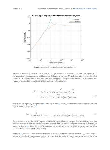
Figure 29. Sensitivity of original and feedback compensated system.

1
Because of unstable , we must add at least a 2 high-pass filter to make stable. But if we append a 2

2
high-pass filter, the compensator will have some DC gain, so we use a 3 high-pass filter to reject the offset

or bias of the acceleration measurement. And also, we append a low-pass filter to reduce the noise effect and
improve robust stability, resulting in that is shown in Equation (27).

1 3 2
=
3
2
2
2
3
0 (1 + ) + 2 1 + 2 + + 2
1 1
2
= 2 3 (27)
3
2
0 (1 + )( + 2 1 + 2 + )( + 2 )
1 1
Finally, we can replace in Equation (20) with Equation (27) to calculate the compensator transfer function,
, as shown in Equation (28).
2
= = (28)
2
1 − 0 (1 + )( + 2 1 + 2 + ) − 2
3
2
2
3
3
1 1
Parameters 1 , 2 are the cutoff frequencies of the high-pass filter and low-pass filter, respectively, and they
must be selected so that the sensitivity of the system is reduced around the peak sensitivity of 80 rad/s, as
shown in Figure 29. Here, the cutoff frequencies are considered across the peak frequency, and we select
1 = 22 rad/s, 2 = 300 rad/s, respectively.
In Figure 30, the Bode diagram shows the response of the overall robot transfer function, , of the original
system and feedback compensated system. It shows that the feedback compensation can reduce the effect