Page 34 - Read Online

Özbek et al. Carbon Footprints 2025, 4, 30 https://dx.doi.org/10.20517/cf.2025.43 Page 13 of 21

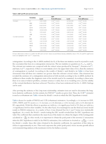
Table 4. ADF and PP unit root test results
ADF PP
Variables
Level First difference Level First difference
***
***
Constant EF -0.81 (0.80) -5.92 (0.00) -0.78 (0.81) -5.94 (0.00)
*** ***
REN 0.74 (0.99) -5.73 (0.00) 1.81 (0.99) -5.75 (0.00)
***
***
GDP 0.60 (0.99) -5.70 (0.00) 0.75 (0.99) -6.17 (0.00)
*** ***
GDP2 0.93 (0.99) -5.60 (0.00) 1.26 (0.99) -5.91 (0.00)
*** ***
NREN -0.08 (0.94) -5.75 (0.00) -0.08 (0.94) -5.75 (0.00)
*** ***
TO -1.91 (0.32) -4.83 (0.00) -1.89 (0.33) -4.83 (0.00)
*** ***
URB -1.10 (0.70) -5.96 (0.00) -1.14 (0.69) -5.96 (0.00)
***
***
Constant and trend EF -1.94 (0.61) -5.86 (0.00) -1.94 (0.61) -5.89 (0.00)
*** ***
REN -1.87 (0.64) -6.12 (0.00) -1.69 (0.73) -9.53 (0.00)
***
*
***
*
GDP -3.26 (0.09) -5.60 (0.00) -3.29 (0.08) -6.05 (0.00)
*** ***
GDP2 -3.07 (0.13) -5.59 (0.00) -3.08 (0.13) -6.15 (0.00)
***
***
NREN -2.00 (0.58) -5.66 (0.00) -2.05 (0.55) -5.66 (0.00)
*** ***
TO -1.32 (0.86) -4.95 (0.00) -1.40 (0.84) -4.96 (0.00)
***
***
URB -1.44 (0.83) -6.01 (0.00) -1.47 (0.82) -6.02 (0.00)
Schwarz information criterion is used in the ADF unit root test. Values in parentheses display probability values. 10%, 5%, and 1% significance
levels are highlighted with * and ***, respectively.
cointegration. According to the A-ARDL method, the H of the three test statistics must be rejected to reach
0
the conclusion that there is a cointegration interaction. The test statistics in question are F , t , and F .
DV
OV
IV
[71]
The relevant test statistics are compared with the critical values produced by Narayan , Pesaran et al. ,
[64]
[65]
and Sam et al. , respectively. If there is a test statistic above the upper limit value of I(1), then the existence
of cointegration is reached. According to the results of Model-1 and Model-2 in Table 5, it has been
determined that all three test statistics are greater than the relevant critical values. This situation has
revealed the existence of a cointegration interaction in both models according to the A-ARDL method. In
addition to these results, the diagnostic tests of the models need to be examined. According to these tests,
there is no autocorrelation problem, constant variance is valid, there is no modeling error, and the validity
of the normal distribution has been achieved. Therefore, it has been understood that the A-ARDL findings
can be used.
After proving the existence of the long-term relationship, estimator tests are used to determine the long-
[56]
term elasticity coefficients. In this context, the FMOLS results are given first. Then, the CCR estimator
[66]
is used as a robustness test. Table 6 shows the Model-1 results in which the EKC hypothesis is tested.
Table 6 shows the results of FMOLS and CCR (robustness) estimators. Accordingly, a 1% increase in GDP,
GDP2, NREN, and TO causes a 2.11% increase, a 0.14% decrease, a 1.08% increase, and a 0.05% decrease in
EF, respectively. While the effects in question are valid at a 10% significance level in TO, they are valid at a
1% significance level in other variables. On the other hand, it is meaningful to use the fixed and trend model
results in FMOLS estimation. As a matter of fact, it was obtained that the C and T terms were statistically
significant. As a result, the Model-1 results testing the EKC model revealed that the EKC hypothesis was
valid. The coefficient that constitutes the main focus of the study is to obtain the degree of the turning point
calculated as . In other words, it is important to obtain the peak point of the inverted-U interaction
when the EKC hypothesis is valid. In the FMOLS estimation, this coefficient is obtained as = 7.53 in
the Model-1 results. Since this value obtained is the elasticity coefficient, the equivalent of this value in
dollars is approximately $1,863. This result expresses the point (peak point) where income growth affects
environmental degradation at the maximum level in the Indian economy.