Page 241 - Read Online

Page 6 of 29 Liu et al. J. Mater. Inf. 2026, 6, 18

where p denotes the total number of features and j the index of the current feature. The scores were
normalized so that their sum equaled unity, enabling the selection of features with cumulative importance
greater than 0.9, which indicated a dominant contribution to property prediction.

After preliminary screening, features were further evaluated using an exhaustive wrapper method to identify
the key subset that governs the strength and ductility of titanium alloys. Considering the distribution of
features, categorical variables were label-encoded, and continuous features standardized via Z-score
normalization. Since the type of target variable determines how the RF iteratively evaluates feature subsets,
the predictive performance of each subset is consequently assessed via repeated training and validation.
Based on these evaluations, the optimal subset is then selected to maximize the coefficient of determination
(R ) while simultaneously minimizing root mean square error (RMSE) for property prediction.
2

Learning algorithm and optimization
According to the “No Free Lunch” (NFL) theorem, no ML algorithm is universally applicable to all
situations. To systematically evaluate model applicability in predicting the strength of titanium alloys at high
strain rates, this work implemented 12 ML algorithms. These include distance-based K-nearest neighbors
(KNNs); kernel-based support vector regression (SVR); tree-based models such as DT and extremely
randomized trees (ExtraTrees); ensemble methods including RF, bootstrap aggregating (Bagging), adaptive
boosting (AdaBoost), gradient boosting regression trees (GBRT), eXtreme gradient boosting (XGBoost),
light gradient boosting machine (LightGBM), and Stacking; as well as a neural network model (artificial
neural network, ANN). R and RMSE were used to evaluate model performance.
2
During model construction, data preprocessing was performed. Data were imported from an Excel file, with
the target variable y defined as the last column and the feature variables X as the remaining columns. Missing
values and outliers were identified and processed. Data integrity and type distribution were assessed through
missing value statistics, followed by descriptive statistical analysis to detect and remove abnormal data
points. In the data partitioning stage, stratified sampling was employed. The standardized dataset was
randomly split into a training set (80%) and a test set (20%), with a random seed of 55 for result
reproducibility. This preprocessing procedure creates a standardized database for model training, enabling
ML algorithms to achieve improved learning and generalization performance.

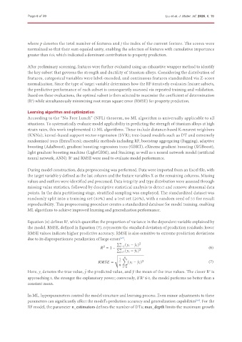
Equation (6) defines R , which quantifies the proportion of variance in the dependent variable explained by
2
the model. RMSE, defined in Equation (7), represents the standard deviation of prediction residuals; lower
RMSE values indicate higher predictive accuracy. RMSE is also sensitive to extreme prediction deviations
due to its disproportionate penalization of large errors .
[67]
Í 2
2 =1 ( − ˆ )
= 1 − Í 2 (6)
=1 ( − ¯ )
v t
1 Õ
= ( − ˆ ) 2 (7)

=1
Here, y denotes the true value, y the predicted value, and y the mean of the true values. The closer R is
2
ˆ
−
i
approaching 1, the stronger the explanatory power; conversely, if R ≤ 0, the model performs no better than a
2
constant mean.
In ML, hyperparameters control the model structure and learning process. Even minor adjustments to these
parameters can significantly affect the model’s prediction accuracy and generalization capabilities . For the
[68]
RF model, the parameter n_estimators defines the number of DTs; max_depth limits the maximum growth