Page 240 - Read Online

Liu et al. J. Mater. Inf. 2026, 6, 18 Page 5 of 29

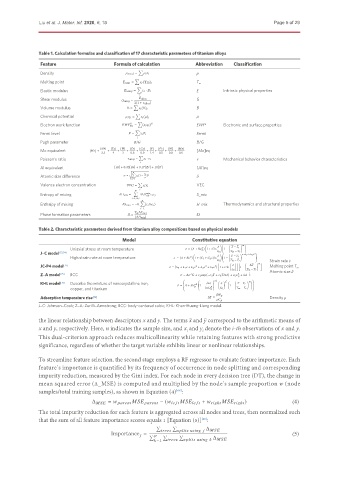
Table 1. Calculation formulas and classification of 17 characteristic parameters of titanium alloys
Feature Formula of calculation Abbreviation Classification
Õ
Density = ρ
Õ
Melting point = (Tm) T m
Õ
Elastic modulus alloy = · E Intrinsic physical properties

Shear modulus alloy = alloy G
2(1 + alloy )
Õ
Volume modulus B = (B) B
Õ
Chemical potential = ( ) μ
Õ
Electron work function = ( ) 6 EWF 6 Electronic and surface properties
6
Õ
Fermi level = Fermi

Pugh parameter / B/G
Mo equivalent [ ] + [ ] + [ ] + [ ] + [ ] + [ ] + [ ] + [ ] + [ ] + [ ] [Mo]eq
3.3 4 2 0.6 0.9 1.4 0.5 0.8 0.6
Õ
Poisson’s ratio alloy = · v Mechanical behavior characteristics

Al equivalent [ ] + 0.33[ ] + 0.17[ ] + 10[ ] [Al]eq
v t
Õ 2
Atomic size difference = (1 − ¯ ) δ
=1
Valence electron concentration VEC = Õ VEC

Õ

Entropy of mixing ΔH mix = 4Δ S_mix
=1, ≠
Õ
Enthalpy of mixing ΔS mix = −R ( ln ) H_mix Thermodynamics and structural properties
=1
Phase formation parameters Ω = Δ Ω
|Δ |
Table 2. Characteristic parameters derived from titanium alloy compositions based on physical models
Model Constitutive equation
¤
Uniaxial stress at room temperature = ( + ) 1 + ln 1 − −

J–C model [73,74] 0 − + 1 ¤ + 2 ¤ 2 !

High strain rate at room temperature = ( + ) 1 + ( 1 + 2 )ln ¤ 1 − −

¤ 0 − Strain rate ε ¤

JC-P4 model [71] = [ 0 + 1 + 2 + 3 + 4 ] 1 + ln ¤ 1 − Δ Melting point T m
2
4
3
¤ 0 − Atomic size δ
Z–A model [75] BCC = Δ + 1 exp(− 3 + 4 ¤) + 5 + − 1 2

0
! 1
KHL model [76] Describe the mixture of nanocrystalline iron, © ¤ ¤ − ª
= ­ + 0 1 − 1 − ®
copper, and titanium 0 ¤ 0 −
« ¬
Adsorption temperature rise [72] Δ = Density ρ

J–C: Johnson–Cook; Z–A: Zerilli–Armstrong; BCC: body-centered cubic; KHL: Khan-Huang-Liang model.
the linear relationship between descriptors x and y. The terms x and y correspond to the arithmetic means of
¯
¯
x and y, respectively. Here, n indicates the sample size, and x and y denote the i-th observations of x and y.
i
i
This dual-criterion approach reduces multicollinearity while retaining features with strong predictive
significance, regardless of whether the target variable exhibits linear or nonlinear relationships.
To streamline feature selection, the second stage employs a RF regressor to evaluate feature importance. Each
feature’s importance is quantified by its frequency of occurrence in node splitting and corresponding
impurity reduction, measured by the Gini index. For each node in every decision tree (DT), the change in
mean squared error (Δ_MSE) is computed and multiplied by the node’s sample proportion w (node
samples/total training samples), as shown in Equation (4) :
[66]
Δ = − ( + ℎ ℎ ) (4)
The total impurity reduction for each feature is aggregated across all nodes and trees, then normalized such
that the sum of all feature importance scores equals 1 [Equation (5)] :
[66]
Í Í
Δ
Í Í
Importance = Í (5)
−1 Δ