Page 92 - Read Online

Page 14 of 20 Gesch et al. J. Mater. Inf. 2025, 5, 42 https://dx.doi.org/10.20517/jmi.2025.23

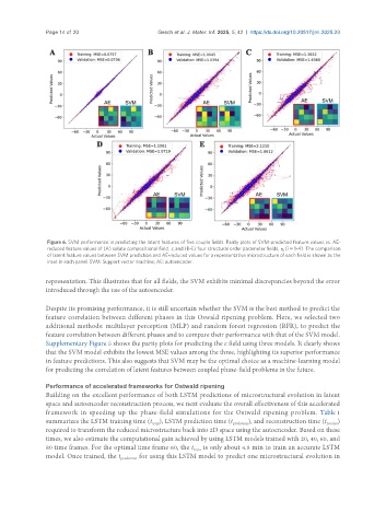
Figure 6. SVM performance in predicting the latent features of five couple fields. Parity plots of SVM-predicted feature values vs. AE-
reduced feature values of (A) solute compositional field, c, and (B-E) four structural order parameter fields, η (i = 1-4). The comparison
i
of latent feature values between SVM prediction and AE-reduced values for a representative microstructure of each field is shown as the
inset in each panel. SVM: Support vector machine; AE: autoencoder.

representation. This illustrates that for all fields, the SVM exhibits minimal discrepancies beyond the error
introduced through the use of the autoencoder.

Despite its promising performance, it is still uncertain whether the SVM is the best method to predict the
feature correlation between different phases in this Oswald ripening problem. Here, we selected two
additional methods: multilayer perception (MLP) and random forest regression (RFR), to predict the
feature correlation between different phases and to compare their performance with that of the SVM model.
Supplementary Figure 5 shows the parity plots for predicting the c field using three models. It clearly shows
that the SVM model exhibits the lowest MSE values among the three, highlighting its superior performance
in feature predictions. This also suggests that SVM may be the optimal choice as a machine-learning model
for predicting the correlation of latent features between coupled phase-field problems in the future.

Performance of accelerated frameworks for Ostwald ripening
Building on the excellent performance of both LSTM predictions of microstructural evolution in latent
space and autoencoder reconstruction process, we next evaluate the overall effectiveness of this accelerated
framework in speeding up the phase-field simulations for the Ostwald ripening problem. Table 1
summarizes the LSTM training time (t ), LSTM prediction time (t prediction ), and reconstruction time (t reconst )
train
required to transform the reduced microstructure back into 2D space using the autoencoder. Based on these
times, we also estimate the computational gain achieved by using LSTM models trained with 20, 40, 60, and
80 time frames. For the optimal time frame 60, the t is only about 4.8 min to train an accurate LSTM
train
model. Once trained, the t prediction for using this LSTM model to predict one microstructural evolution in