Page 89 - Read Online

Gesch et al. J. Mater. Inf. 2025, 5, 42 https://dx.doi.org/10.20517/jmi.2025.23 Page 11 of 20

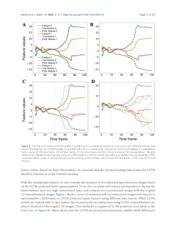
Figure 4. Training performance of LSTM models in predicting the evolution of reduced microstructure with different training time
frames. The training loss of LSTM models for predicting the top four autoencoder-reduced microstructural features of compositional
field, c, using (A) 80 time frames, (B) 60 time frames, (C) 40 time frames, and (D) 20 time frames as the training dataset. The grey
dashed lines indicate the starting time frame for LSTM prediction, and the dotted lines after grey dashed lines represent the LSTM-
predicted feature values of reduced microstructure evolving as time frames until the last 100 time frame. LSTM: Long short-term
memory.

feature values. Based on these observations, we conclude that the optimal training time frames for LSTM
models is between 40-60 for Ostwald ripening.

With the optimal time frames, we next evaluate the accuracy of reconstructed microstructure images based
on the LSTM-predicted latent representations. To do this, we adopt well-trained autoencoders to decode the
latent features back into high-dimensional space and compare the reconstructed images with the original
2D microstructural images. Figure 5 shows a series of reconstructed microstructural images over time for a
representative c field based on LSTM-predicted latent features using different time frames. When LSTM
models are trained with 70 time frames, the reconstructed microstructures using LSTM-reduced features are
almost identical to the original 2D images. This similarity is supported by the pointwise error plots in the
third row of Figure 5B, which shows that the LSTM-predicted microstructures exhibit small differences