Page 93 - Read Online

Gesch et al. J. Mater. Inf. 2025, 5, 42 https://dx.doi.org/10.20517/jmi.2025.23 Page 15 of 20

Table 1. Performance of accelerated phase-field frameworks using different LSTM models
LSTM time frames t train (min) t prediction (s) t reconst (s) Computational gain
20 4.3 0.046 0.772 3.54 × 10 5
5
40 4.8 0.042 0.589 3.44 × 10
5
60 4.2 0.033 0.400 3.35 × 10
80 2.6 0.018 0.246 2.74 × 10 5
t is the time for training one LSTM model. t is the time for predicting the future sequence using LSTM model. t is reconstruction
train prediction reconst
time by using autoencoder to transform latent microstructure back to high-dimensional space. Computational gain is the speed up of using
accelerated framework to generate a microstructure image as part of an evolution compared to phase-field simulations. LSTM: Long short-term
memory.

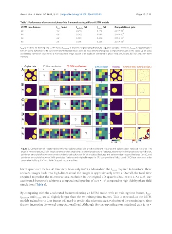
Figure 7. Comparison of reconstructed microstructure using SVM-predicted latent features and autoencoder-reduced features. The
original microstructure, SVM input parameters for predicting latent microstructural features, reconstructed microstructure prediction,
pointwise error plots between reconstructed microstructures of SVM-predicted features and autoencoder-reduced features (ideal), and
pointwise error plots between SVM-predicted features and original images for (A) compositional field, c, and (B-E) four structural order
parameter fields, η (i = 1-4). SVM: Support vector machine.
i
latent space over the last 40 time steps takes only 0.033 s. Meanwhile, the t reconst required to transform these
reduced images back into high-dimensional 2D images is approximately 0.772 s. Overall, the total time
required to predict the microstructural evolution in the original 2D space is about 0.818 s. As such, our
accelerated framework achieves a computational speedup of 3.35 × 10 compared to high-fidelity phase field
5
simulations [Table 1].

By comparing with the accelerated framework using an LSTM model with 40 training time frames, t ,
train
t prediction , and t reconst are all slightly longer than the 60 training time frames. This is expected, as the LSTM
models trained on 40 time frames will need to predict the microstructual evolution of the remaining 60 time
frames, increasing the overal computational load. Although the corresponding computational gain (3.44 ×