Page 85 - Read Online

Gesch et al. J. Mater. Inf. 2025, 5, 42 https://dx.doi.org/10.20517/jmi.2025.23 Page 7 of 20

type by using only these 16 values in latent space. The pointwise error of 2D images was plotted to visualize
the difference between autoencoder-reconstructed 2D images and original ones, and the method for
[50]
plotting pointwise error has been discussed in Ref. .

Machine-learning engine of microstructural evolution
Another key component of this accelerated phase-field framework is the machine learning engine, which
learns the dynamics of microstructure evolution within the latent representation space. As history-
dependent machine learning techniques, RNN models have been widely adopted as the preferred machine
learning engines to accelerate microstructure predictions [45-49] . RNNs are a class of artificial neural networks
that use time series data, or sequential data, to predict future data values . In this work, the reduced
[67]
microstructures of five interdependent phase fields in Ostwald ripening were individually treated as time-
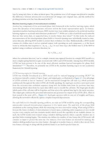
series data sets, allowing RNN models to predict their evolution over time. Mathematically, a RNN model
consists of a hidden state h and an optional output, both operating on each component, x, of the latent
t
vector x within the time sequence x = (x , x , ..., x ). At each time step t, the hidden state h of the RNN is
2
t
N
t
1
updated using a nonlinear activation function f as:
(6)
where the activation function f can be a simple element-wise sigmoid function in a simple RNN model or a
more complex gating function in gate recurrent unit (GRU) and LSTM models. Among these RNN models,
LSTM has been proven to be one of the most efficient machine-learned surrogates for phase-field
simulations [46,47,49] . Therefore, we primarily use LSTM as the machine learning engine in our accelerated
framework for Ostwald ripening.

LSTM learning engine for Ostwald ripening
LSTM was initially introduced as a RNN model used for natural language processing (NLP) . Its
[68]
architecture typically consists of input, forget, and output gates, as illustrated in Figure 1C. One advantage
of LSTM network is that its “memory” can be maintained through the cell state (c), which performs
t
continuously throughout the entire LSTM cell. Briefly speaking, the input gate receives a new input point
from the microstructure evolution sequence along with the hidden state from the previous time step,
determining which values from the input data will be used to modify the cell state. The forget gate decides
which parts of the cell state will be forgotten and thus selects the optimal time lag for the input sequence.
The output gate combines the processed information and generates the output of the LSTM cell h, which is
t
then passed to the next cell h [Figure 1C]. Each gate operates with its own set of weights and biases,
t+1
allowing the network to effectively capture complex temporal dependencies.

For each field in this Ostwald ripening problem, we train an LSTM model by using the corresponding
autoencoder-reduced microstructure sequences in the latent space. We used 80% of the phase-field
simulations as the training dataset, while the remaining 20% were reserved for testing. When using LSTM to
forecast the future evolution of microstructure in latent space, predicting entire sequences at once would
require a very complex and data-intensive model, which exceeds the capability of our available dataset. As
such, the LSTM models were trained using a window-shifting method, where a specific window size is
specified before training begins. This window size defines the number of time frames the LSTM model will
consider as input to predict the next one. For instance, if 80 time frames are selected for training, the
window-shifting method uses true time frames 1 through 80 to predict frame 81, which is then stored. Next,
true frames 2 through 80 along with the predicted frame 81 are used to predict frame 82.