Page 83 - Read Online

Gesch et al. J. Mater. Inf. 2025, 5, 42 https://dx.doi.org/10.20517/jmi.2025.23 Page 5 of 20

[52]
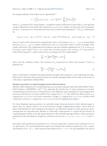
free energy landscape of the system can be expressed by :
(2)

where f is chemical free energy density, κ is gradient energy coefficient for solute field, κ is the gradient
η
c
chem
energy coefficients for structural order parameters η , and p is the number of structural order parameters.
p
We set p = 4 because it is a commonly used value used in nickel-based superalloys . The f is determined
[52]
chem
by:
(3)
α
β
where f and f are the chemical free energy density of the α and β phases, h (η , η , ..., η ) is an interpolation
2
1
p
function, g (η , η , ..., η ) is a double-well function, and w is a parameter which controls the height of the
p
2
1
β
α
double-well barrier. The mathematical formulations and more detailed explanations for f , f , h, and g can
be found in prior study . Since c (x, t) must obey contiuity equation, the evolution of c is governed by
[52]
Cahn-Hilliard equation , which is derived from an Onsager force-flux relationships :
[53]
[5]
(4)
where M is the mobility of solute. The evolution of η is governed by Allen-Cahn equation based on
[54]
p
gradient flow:
(5)
where L is the kinetic coefficient associated with the structural order parameter η . By considering one solute
p
field and four structural order parameter fields, the Ostwald ripening problem in this study can be treated as
a five-phase coupled phase-field problem.

Database generation via high-throughput phase-field simulations
All phase-field simulations for Ostwald ripening were performed using the Mesoscale Mutli-Physics Phase-
Field Simulator (MEMPHIS) code [55,56] . By analyzing the distribution of input parameters and their
corresponding microstructures, we found that the most influential input parameters for generating diverse
microstructural features are solute mobility (M), ranging from 4.5 to 5, the equilibrium phase fraction (c ),
α
ranging from 0.15 to 0.45, the initial composition average (c ), ranging from 0.45 to 0.55, and the initial
0
composition variance (ϵ), ranging from 0.04 to 0.08, as shown in Supplementary Figure 1.

For these dominant input parameters, we randomly sample these parameters in their optimal ranges to
ensure they can capture a diverse set of microstructure images. Supplementary Figure 1 shows that 200
phase-field simulations with varying input parameters can effectively sample the entire parameter space,
ensuring that our microstructure database is sufficiently comprehensive to capture the key features of
coupled parameter fields across the spatial domain for this Ostwald ripening problem. Other parameters
necessary for the simulation are adopted as constants, and they are: κ = κ = 3, ρ = , w = 1, α = 5, and L =
η
c
[52]
5 .
Each phase-field simulation was performed on a 2D square grid with a uniform mesh composed of 256 ×
256 grid points. We used dimensionless spatial and temporal discretization parameters, with a spatial
discretization of Δx = Δy = 1, and a temporal discretization of Δt = 1 × 10 . For each simulation, the total of
-3