Page 49 - Read Online

Allen et al. J Mater Inf 2024;4:35 https://dx.doi.org/10.20517/jmi.2024.72 Page 9 of 15

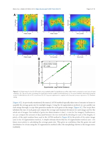
Figure 2. (A) Heat maps for the BO-GP model using inverted scaled Fréchet distance as the output metric projected on each pair of input
variables; (B) The parity plot comparing the predicted inverted scaled Fréchet distances vs. the experimentally determined inverted
scaled Fréchet distance for all PC conditions. BO-GP: Bayesian optimization coupled with Gaussian process regression; PC: Photonic
curing.

[Figure 3C]. As previously mentioned, the manual ASTM method typically takes tens of minutes to hours to
quantify the average grain size for multiple images. Using the AI segmentation method, we can quickly run
each image through a script that generates masks for each grain in the image [Figure 3C]. The script then
tabulates the size of each grain and outputs the average and standard deviation for each image and for the
whole set of images. Our method of grain size determination is fast (~3 min for five images). Furthermore,
we can compare the amount of data used between the two methods by dividing the sum of the lengths, in
pixels, of the eight random lines used in the ASTM method in Figure 3B by the pixels of the entire image
used in the AI segmentation method. A simple estimate shows that the AI segmentation method uses ~200
times more pixels in calculating the average grain size. This gives us confidence that the grain size and
distribution we obtain using the AI segmentation method reflect the morphology shown in the images more
truthfully.