Page 45 - Read Online

Allen et al. J Mater Inf 2024;4:35 https://dx.doi.org/10.20517/jmi.2024.72 Page 5 of 15

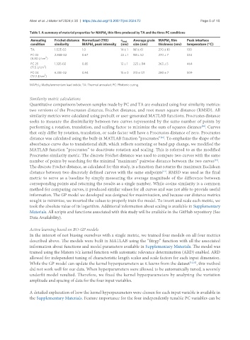
Table 1. A summary of material properties for MAPbI thin films produced by TA and the three PC conditions
3
Annealing Fréchet distance Normalized (110) σ RMS Average grain MAPbI film Peak interface
3
condition similarity MAPbI peak intensity (nm) size (nm) thickness (nm) temperature (°C)
3
TA 1.02E-02 1.0 14 ± 1 161 ± 61 270 ± 10 100
PC 03 2.84E-02 0.67 22 ± 1 151 ± 52 270 ± 7 334
2
(6.80 J/cm )
PC 25 1.32E-02 0.85 12 ± 1 223 ± 84 263 ± 5 464
2
(11.5 J/cm )
PC 04 6.35E-02 0.94 15 ± 0 313 ± 121 280 ± 7 509
2
(12.2 J/cm )
MAPbI : Methylammonium lead iodide; TA: Thermal annealed; PC: Photonic curing.
3
Similarity metric calculations
Quantitative comparisons between samples made by PC and TA are evaluated using four similarity metrics:
two versions of the Procrustes distance, Fréchet distance, and root mean square distance (RMSD). All
similarity metrics were calculated using prebuilt or user-generated MATLAB functions. Procrustes distance
seeks to measure the dissimilarity between two curves represented by the same number of points by
performing a rotation, translation, and scaling factor to minimize the sum of squares distance . Curves
[28]
that only differ by rotation, translation, or scale factor will have a Procrustes distance of zero. Procrustes
distance was calculated using the built-in MATLAB function “procrustes” . To emphasize the shape of the
[29]
absorbance curve due to translational shift, which reflects scattering or band gap change, we modified the
MATLAB function “procrustes” to deactivate rotation and scaling. This is referred to as the modified
Procrustes similarity metric. The discrete Fréchet distance was used to compare two curves with the same
number of points by searching for the minimal “maximum” pairwise distance between the two curves .
[30]
The discrete Fréchet distance, as calculated for this study, is a function that returns the maximum Euclidean
distance between two discretely defined curves with the same endpoints . RMSD was used as the final
[31]
metric to serve as a baseline by simply measuring the average magnitude of the difference between
corresponding points and returning the results as a single number. While cosine similarity is a common
method for comparing curves, it produced similar values for all curves and was not able to provide useful
information. The GP model we developed was designed for maximization, and because our distance metrics
sought to minimize, we inverted the values to properly train the model. To invert and scale each metric, we
took the absolute value of its logarithm. Additional information about scaling is available in Supplementary
Materials. All scripts and functions associated with this study will be available in the GitHub repository (See
Data Availability).

Active learning based on BO-GP models
In the interest of not biasing ourselves with a single metric, we trained four models on all four metrics
described above. The models were built in MATLAB using the “fitrgp” function with all the associated
information about functions and model parameters available in Supplementary Materials. The model was
trained using the Matern 5/2 kernel function with automatic relevance determination (ARD) enabled. ARD
allowed for independent tuning of characteristic length scales and scale factors for each input dimension.
While the GP model can update the kernel hyperparameters as it learns from the dataset [12,32] , this method
did not work well for our data. When hyperparameters were allowed to be automatically tuned, a severely
underfit model resulted. Therefore, we fixed the kernel hyperparameters by analyzing the variation
amplitude and spacing of data for the four input variables.

A detailed explanation of how the kernel hyperparameters were chosen for each input variable is available in
the Supplementary Materials. Feature importance for the four independently tunable PC variables can be