Page 103 - Read Online

Li et al. Intell Robot 2022;2(1):89–104 I http://dx.doi.org/10.20517/ir.2022.02 Page 97

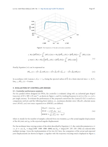
Figure 4. Test trajectory of the pick-and-place operation.

∫ ∫
®
®
®
≤ (k (0)k + k ® ( )kd ) + (k +1 (0)k + k (0)k + k ® ( )kd
0 0
( ∫ )
®
®
≤ max(1, + ) k +1 (0)k + k (0)k + k ® ( )kd (34)
0
Finally, Equation (33) can be expressed as:
® ® ® ® ® ® ® ® (35)
® +1 ( ) = ( + )( ® )( ) = ( + )( + −1 ) · · · ( + 0 )( ® 0 )( )

In accordance with Lemma 2, if < 1, being the spectral radius of , for a finite interval time ∈ [0, ],
®
lim →∞ ® +1 ( ) = 0 exists.

5. EVALUATION OF CONTROLLER DESIGN
5.1. Controller performance analysis
For the parallel robots designed for PPOs, the controller is evaluated along with an industrial gate-shaped
[6]
trajectory of 25 × 305 × 25 mm , as shown in Figure 4, and the working frequency is set to 2 Hz, i.e., 0.25 s
per single journey. To evaluate the performance of the proposed control law, the classical D-ILC is used as a
comparison method, and the following three indices, i.e., maximum absolute error ( ), absolute mean
error ( ), and root-mean-squared error ( ), are defined:


 = max(| − |)


 1 ∑
= | − | (36)
=1
 √
 ∑
 1 2
 = ( − )
 =1
where stands for the number of samples collected from one iteration, is the actual angular displacement
of the th joint, and is the expected angular displacement.
For the nonlinear time-varying system of the robot described by Equation (17), the controller parameters =
1.1, = 1.22, = diag([1000 1000 1000 1000] and = diag([230 230 230 230]) are selected after
multiple tunings. Upon the implementation of the two ILC laws, the comparison of the actual and expected
joint displacements are shown in Figure 5, together with the trajectory tracking results displayed in Figure 6.