Page 30 - Read Online

Page 12 of 16 Zander et al. Complex Eng Syst 2023;3:9 I http://dx.doi.org/10.20517/ces.2023.11

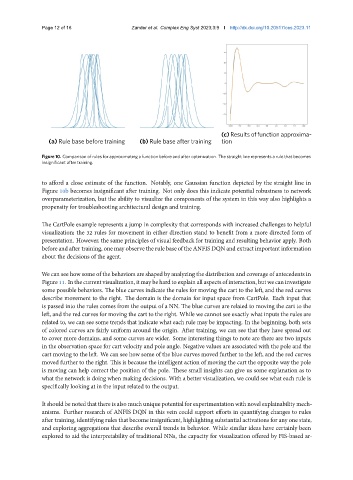
(c) Results of function approxima-
(a) Rule base before training (b) Rule base after training tion

Figure 10. Comparison of rules for approximating a function before and after optimization. The straight line represents a rule that becomes
insignificant after training.

to afford a close estimate of the function. Notably, one Gaussian function depicted by the straight line in
Figure 10b becomes insignificant after training. Not only does this indicate potential robustness to network
overparameterization, but the ability to visualize the components of the system in this way also highlights a
propensity for troubleshooting architectural design and training.

The CartPole example represents a jump in complexity that corresponds with increased challenges to helpful
visualization; the 32 rules for movement in either direction stand to benefit from a more directed form of
presentation. However, the same principles of visual feedback for training and resulting behavior apply. Both
before and after training, one may observe the rule base of the ANFIS DQN and extract important information
about the decisions of the agent.

We can see how some of the behaviors are shaped by analyzing the distribution and coverage of antecedents in
Figure11. Inthecurrentvisualization,itmaybehardtoexplainallaspectsofinteraction,butwecaninvestigate
some possible behaviors. The blue curves indicate the rules for moving the cart to the left, and the red curves
describe movement to the right. The domain is the domain for input space from CartPole. Each input that
is passed into the rules comes from the output of a NN. The blue curves are related to moving the cart to the
left, and the red curves for moving the cart to the right. While we cannot see exactly what inputs the rules are
related to, we can see some trends that indicate what each rule may be impacting. In the beginning, both sets
of colored curves are fairly uniform around the origin. After training, we can see that they have spread out
to cover more domains, and some curves are wider. Some interesting things to note are there are two inputs
in the observation space for cart velocity and pole angle. Negative values are associated with the pole and the
cart moving to the left. We can see how some of the blue curves moved further to the left, and the red curves
moved further to the right. This is because the intelligent action of moving the cart the opposite way the pole
is moving can help correct the position of the pole. These small insights can give us some explanation as to
what the network is doing when making decisions. With a better visualization, we could see what each rule is
specifically looking at in the input related to the output.

It should be noted that there is also much unique potential for experimentation with novel explainability mech-
anisms. Further research of ANFIS DQN in this vein could support efforts in quantifying changes to rules
after training, identifying rules that become insignificant, highlighting substantial activations for any one state,
and exploring aggregations that describe overall trends in behavior. While similar ideas have certainly been
explored to aid the interpretability of traditional NNs, the capacity for visualization offered by FIS-based ar-