Page 29 - Read Online

Zander et al. Complex Eng Syst 2023;3:9 I http://dx.doi.org/10.20517/ces.2023.11 Page 11 of 16

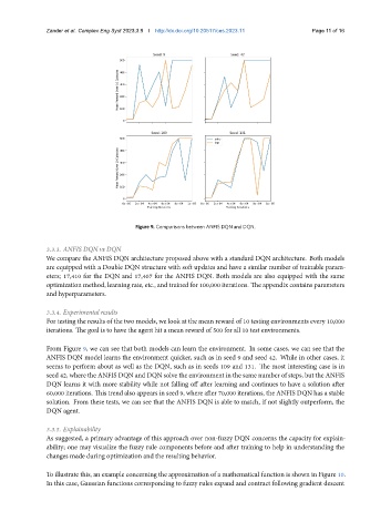
Figure 9. Comparisons between ANFIS DQN and DQN.

3.3.3. ANFIS DQN vs DQN
We compare the ANFIS DQN architecture proposed above with a standard DQN architecture. Both models
are equipped with a Double DQN structure with soft updates and have a similar number of trainable param-
eters; 17,410 for the DQN and 17,407 for the ANFIS DQN. Both models are also equipped with the same
optimization method, learning rate, etc., and trained for 100,000 iterations. The appendix contains parameters
and hyperparameters.

3.3.4. Experimental results
For testing the results of the two models, we look at the mean reward of 10 testing environments every 10,000
iterations. The goal is to have the agent hit a mean reward of 500 for all 10 test environments.

From Figure 9, we can see that both models can learn the environment. In some cases, we can see that the
ANFIS DQN model learns the environment quicker, such as in seed 9 and seed 42. While in other cases, it
seems to perform about as well as the DQN, such as in seeds 109 and 131. The most interesting case is in
seed 42, where the ANFIS DQN and DQN solve the environment in the same number of steps, but the ANFIS
DQN learns it with more stability while not falling off after learning and continues to have a solution after
60,000 iterations. This trend also appears in seed 9, where after 70,000 iterations, the ANFIS DQN has a stable
solution. From these tests, we can see that the ANFIS DQN is able to match, if not slightly outperform, the
DQN agent.

3.3.5. Explainability
As suggested, a primary advantage of this approach over non-fuzzy DQN concerns the capacity for explain-
ability; one may visualize the fuzzy rule components before and after training to help in understanding the
changes made during optimization and the resulting behavior.

To illustrate this, an example concerning the approximation of a mathematical function is shown in Figure 10.
In this case, Gaussian functions corresponding to fuzzy rules expand and contract following gradient descent