Page 57 - Read Online

Hu et al. J. Mater. Inf. 2025, 5, 44 https://dx.doi.org/10.20517/jmi.2025.21 Page 7 of 17

(3) Prediction MLP: BN is also applied to the prediction MLP; however, the output fully connected layer is
not followed by BN or ReLU activation. This MLP comprises two fully connected layers, with the first layer
having input and output dimensions of 2,048, and the second layer having an output dimension of 512.

The NEU dataset was subjected to pre-training across a range of 100-800 epochs, employing a batch size of
64 and a learning rate of 0.1. This process yielded eight distinct sets of pre-trained weights, designated as
NEU-100e to NEU-800e. Concurrently, the SSDD dataset underwent pre-training for 100-400 epochs,
yielding four unique sets of pre-trained weights, designated as SSDD-100e to SSDD-400e, with a batch size
of 128 and a learning rate of 0.2. Furthermore, the amalgamated SSDD + NEU dataset was pre-trained for
100 and 200 epochs, yielding two additional sets of pre-trained weights, termed SSDD + NEU-100e and
SSDD + NEU-200e. Subsequently, the aforementioned pre-trained weights are applied to the downstream
tasks for object detection.

For object detection, we selected Faster R-CNN [Figure 3B] - a two-stage framework that generates region
[42]
proposals before classification/refinement. Its multi-scale detection capability and proven accuracy suit
defect detection tasks prioritizing precision over speed.

[43]
We implement Faster R-CNN with ResNet18 [Figure 4] as the backbone. To preserve generic features
while adapting to defects:
Stage 0 freezes the initial feature extractors: conv1 (7 × 7 convolution), bn1 (BN), ReLU activation, and
maxpool (3 × 3 max pooling).
Stage 1 freezes the first residual group: layer1 (containing four 3 × 3 convolutions with two skip
connections).

This allows layers 2-4 to fine-tune defect-specific patterns, leveraging transfer learning from pre-trained
weights.

In Faster R-CNN, the region proposal network (RPN) processes the backbone-generated feature map to
filter anchor boxes and generate region proposals. The RPN classifies regions as foreground (object-
containing) or background but cannot identify object categories. During the second stage, positive
proposals and corresponding feature map regions undergo ROI Pooling for dimensional standardization
before entering the ROI Head. Here, convolutional and fully connected layers classify objects and refine
bounding box coordinates to produce final detections.

Evaluation index
Quantitative evaluation of steel surface defect detection methods employed two primary metrics: mean
average precision (mAP) and mAP at intersection over union (IoU) threshold 0.5 (mAP_50).

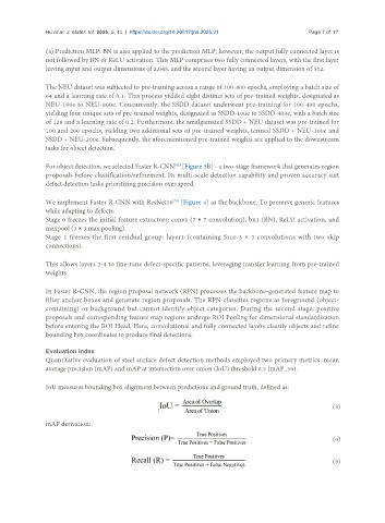
IoU measures bounding box alignment between predictions and ground truth, defined as:

(3)

mAP derivation:

(4)

(5)