Page 67 - Read Online

Page 8 of 19 Tang et al. J. Mater. Inf. 2025, 5, 38 https://dx.doi.org/10.20517/jmi.2025.05

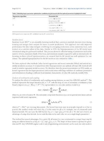
Table 1. Modeling hyper-parameter optimization candidates by grid search with the optimal parameters highlighted in bold
Regression algorithm Parameter list
SVR C: 0.1, 1, 10, 100,1000
Kernel function: RBF
gamma γ: 0.001, 0.01, 0.1, 0.5
RF n_estimators: 20, 50, 70
max_depth: 3, 4, 5, 7, 10
min_samples_split: 2, 4, 6, 10

SVR: Support vector regression; RBF: radial basis function; RF: random forest.

Random forest
Random forest (RF) is an ensemble learning method that constructs multiple decision trees during
[46]
training and merges their outputs for more accurate predictions. This approach not only improves
performance but also helps mitigate overfitting by averaging predictions across numerous trees, each
trained on a random subset of the data. Similar to SVR, the hyperparameters of the RF model were
determined using the grid search method. This process allows for efficient tuning of parameters such as the
number of trees, maximum depth of the trees, and minimum samples required to split an internal node. By
focusing on these critical hyperparameters, we ensured that the RF model was well-optimized for our
dataset. The optimal hyperparameters for the RF model are also outlined in Table 1.

We have explored other methods [other kernel regressions and neural networks (NNs)] and arrived at a
similar prediction accuracy. It is natural that when hyperparameters are optimal, all major ML methods will
result in similar regression model accuracy. We therefore limit the present presentation to SVR results, as
kernel regression has few hyperparameters and avoids issues with large numbers of nonlinear parameters
and initializations (leading to different local minima) characteristic of other ML methods, notably NNs.

Analysis of nonlinearity and coupling
To analyze the effects of nonlinearity and coupling among features, we used the GPR-NN method . The
[47]
method represents the target function f(x), x ∈ R , with the help of a set of redundant coordinates y that
D
N>D
linearly depend on x, y = Wx, y ∈ R . The representation is a 1st order additive model in y:
(6)

where w are rows of matrix W. The univariate component functions f (y ) are in general non-linear and are
n
n
n
expressed with kernel regression,
(7)

(m)
where y = Wx are training data points. The kernel functions may in principle depend on n, but in
(m)
practice the method works well when k(χ, χ′) is the same for all n, for example, one of commonly used
2
2
Matern kernels. We use here the RBF kernel k(χ, χ′) = exp(-2l (χ, χ′) ) for all n. We did not observe an
advantage of using other kernels. As we scale the data on the unit cube, we use a single length parameter l.
The method has several advantages. For a given W, all terms f (y ) are constructed in a single linear step by
n
n
2
N
using an additive kernel in y, k(y, y′) = Σ exp(-2l (y -y′ ) ). The shape of these terms is optimal for given
2
n=1
n
n
data and W. Any GPR/KRR engine (code in any programming environment) can be used, one only needs to