Page 66 - Read Online

Tang et al. J. Mater. Inf. 2025, 5, 38 https://dx.doi.org/10.20517/jmi.2025.05 Page 7 of 19

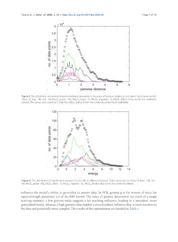
Figure 3. The distribution of pairwise distances between datapoints in the space of features (scaled on unit cube). Solid curves are for
alloys of: blue - Nb, red - Nb -Nb Si , green - Nb -Nb Si , black - Si -Nb Si , magenta - Si -Nb Si . Black circles are for the combined
3
I
5
3
II
3
II
5
5
3
5
I
dataset. The curves were scaled by 1/3 for Nb -Nb Si and by 1/6 for the combined set for better readability.
3
5
II

Figure 4. The distribution of substitution energies (in eV/cell) in different datasets. Solid curves are for alloys of: blue - Nb, red -
Nb -Nb Si , green - Nb -Nb Si , black - Si -Nb Si , magenta - Si -Nb Si . Black circles are for the combined dataset.
I 5 3 II 5 3 I 5 3 II 5 3

influence the model’s ability to generalize to unseen data. In SVR, gamma g is the inverse of twice the
squared length parameter (σ) of the RBF kernel. The value of gamma determines the reach of a single
training example: a low gamma value suggests a far-reaching influence, leading to a smoother, more
generalized model, whereas a high gamma value implies a more localized influence that is more sensitive to
the data and potentially more complex. The results of this optimization are detailed in Table 1.