Page 54 - Read Online

Li et al. J Mater Inf 2024;4:4 I http://dx.doi.org/10.20517/jmi.2023.41 Page 9 of 14

Table 2. The structure of local environment ResNet
Layer name Output size 34-Layer
Conv1 6 × 11 1 × 1, 32, stride 1
" #
3 × 3, 32
Conv2_x 6 × 11 3 × 3, 32 × 3, stride 1
" #
3 × 3, 64
Conv3_x 3 × 6 3 × 3, 64 × 4, stride 2
" #
3 × 3, 128
Conv4_x 2 × 3 3 × 3, 128 × 6, stride 2
" #
3 × 3, 256
1 × 2 × 3, stride 2
Conv5_x 3 × 3, 256
1 × 1 AdaptiveAvgPool

0.4 split
train
test
0.2

0
residual −0.2

−0.4

−0.6

−2 0 2 4
prediction

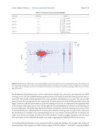
Figure 3. Residual plot of LERN models. The left-hand side is a scatter plot, where the x-axis is the predicted value of the model on the
training and test sets, the y-axis is the corresponding predicted value minus the true value, and the middle corresponds to its regression
line, respectively. On the right-hand side are the residual distributions for the training and test sets, respectively. LERN: Local environment
input into ResNet.

the distribution of prediction errors. In the scatter plot on the left, the x-axis and y-axis represent the LERN
training process and the residuals between predicted and actual values on both the training and test sets, re-
spectively. The overall residual regression line is also calculated and displayed in the plot. The red and blue
parts represent the training and test sets, respectively. It can be observed that the LERN prediction results are
highly consistent with the actual values on both the training and test sets, as evidenced by the regression lines
of the residuals with slopes close to zero. On the right, the overall distribution of residuals on the training and
testsetsisdisplayed. Theresultsshowthatthedistributionofresidualsonboththetrainingandtestsetsisclose
to normal distribution, indicating that the model is well-suited for learning from this type of data. Moreover,
the distributions of residuals on the training and test sets are very similar, indicating that the model does not
suffer from obvious overfitting. Therefore, the LERN prediction results are highly consistent with the actual
DFT calculation results within the allowable error range, suggesting that LERN has DFT-level accuracy.

To benchmark the performance of our proposed model in a materials database, we use other state-of-the-art
[6]
neural networks. We compare our LERN with the original CGCNN, SchNet [57] , AliGNN , and our Modified