Page 45 - Read Online

Page 238 Yang et al. Intell Robot 2022;2(3):223­43 I http://dx.doi.org/10.20517/ir.2022.19

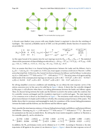
Figure 2. The communication topology graph.

A discrete semi-Markov jump process with semi-Markov kernel is employed to describe the switching of
topologies. The transition probability matrix of EMC and the probability density function of sojourn time
are provided by

 0 0.8 0.2   0 0.6 ·0.4 (10− ) ·10! 0.7 ·0.3 (10− ) ·10!
(10− )! !
(10− )! !
    1.8 1.8 10  
[ ] = 0.26 0 0.74 , [ ( )] = 0.4 ( −1) − 0.4 0 0.5 10!  .


  (10− )! !
 
 0.5 0.5 0   ( −1) 1.3 1.3 ( −1) 1.5 1.5 
  0.5 − 0.5 0.4 − 0.4 0
 
1
2
3
Let the upper bound of the sojourn-time for each topology mode be = = = 5. The statistical
characteristicparametersofchannelfadingareselectedas 1 = 0.8, 2 = 0.7, 3 = 0.75, 01 = 0.75, 02 = 0.85,
03 = 0.6, 1 = 0.05, 2 = 0.15, 3 = 0.2, 01 = 0.1, 02 = 0.25, 03 = 0.15.
First, we assume that there is no channel fading phenomenon between the leader and the follower, that is,
( ) = 1 and 0 ( ) = 0 in system (6). In this case, mean square consensus conditions in Theorem 2 will be
somewhat simplified. At this time, the channel interference between the follower and the follower is selected as
] . The initial states of all agents and the
( ) = [0.02 sin( ) (−0.1 ) 0.01 cos( ) (−0.1 ) − 0.01 sin( ) (−0.1 )

initial mode of the communication topology are chosen as 0 (0) = [0.2 − 0.1 0.2] , 1 (0) = [0.1 − 0.3 0.4] ,
2 (0) = [−0.4 0.8 − 0.2] , 3 (0) = [0.5 − 0.2 0.4] , 4 (0) = [0.3 − 0.6 − 0.1] , and ( ) = 1.

By solving simplified consensus conditions and simulating, we can obtain the state response curves of the
system consensus error in this case as the solid line in Figure 3 shown. It shows that the controller designed
in this paper is still effective when there is no fading phenomenon between the leader and follower agents.
Then, the channel fading between the leader and the follower is added to the system under the condition that
the controller remains unchanged, and the simulation experiment is performed again. The state trajectory
of the consensus error is shown as the dotted line in Figure 3. The simulation results indicate that the fading
phenomenonbetweentheleaderandthefollowerwillaffecttheconsensusandperformanceofthesystem. This
further shows that it is necessary and meaningful to study the coexistence of the channel fading phenomenon
between the leader and the follower, and the follower and the follower agent.
Next, consider thesimultaneous existence of channel fading between leader and follower and between follower
] . The rest of
and follower. Choosing 0 ( ) = [−0.01 sin( ) (−0.1 ) 0.01 cos( ) (−0.1 ) 0.02 sin( ) (−0.1 )
the parameters are the same as stated above. By solving the linear matrix inequality condition in Theorem 2,
the controller gains can be calculated as

[ ] [ ] [ ]
2.3702 1.1042 −2.6922 3.7920 1.9250 −4.7775 2.2009 1.2900 −3.1491
1 = , 2 = , 3 =
0.8871 0.8304 −0.9780 1.4275 1.3860 −1.7717 0.8326 0.9225 −1.1972
In addition, the H ∞ performance index can be obtained as ˆ = 2.3705. According to Theorem 2, the state
trajectories of all agents in the system (6) are shown in Figure 4. Figure 5 shows the state-response curves of