Page 123 - Read Online

Page 307 Peng et al. Intell Robot 2022;2(3):298­312 I http://dx.doi.org/10.20517/ir.2022.27

Table 1. Configuration of three-area power systems
ℎ ( ) ( ) ( )
1 0.30 0.37 0.05 1.0 1 1 + 1 10
2 0.17 0.40 0.05 1.5 2 4 + 2 10
3 0.20 0.35 0.05 1.8 3 + 3 12
3
12 = 0.20, 13 = 0.12, 23 = 0.25( / )

0.5

0.25

0

-0.25

-0.5

-0.75

-1

-1.25

-1.5
0 5 10 15 20

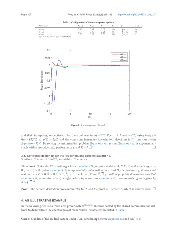
Figure 2. State responses of case 1.

−1
and their transposes, respectively. For the nonlinear terms − ˜ −1 , = 1, 2 and − , using inequali-

2 ˜
ties − ˜ −1 ≤ − 2 and the cone complementary linearization algorithm in [27] , one can obtain

(32) . By solving the minimization problem Equation (31), system Equation (12) is exponentially
∗
stable with a prescribed ∞ performance and = ℶ . □
−1
3.4. Controller design under the RR scheduling scheme Equation (7)
Similar to Theorem 5.2 in [29] , we establish Theorem 4.
Theorem 4 Under the RR scheduling scheme Equation (7), for given matrices , , , , and scalars , >
0, > 0, > 0, system Equation (12) is exponentially stable with a prescribed ∞ performance , if there exist
real matrices > 0, > 0, > 0, > 0, = 1, · · · , and ,ℶ, with appropriate dimensions such that
˜
˜
˜
˜
Equation (31) is solvable with = , where is given by Equation (30). The controller gain is given by
−1
= ℶ .
−1
Proof: The detailed derivation process can refer to [29] and the proof of Theorem 3, which is omitted here. □

4. AN ILLUSTRATIVE EXAMPLE
In the following, we use a three-area power system [23,24,28] interconnected by the shared communication net-
work to demonstrate the effectiveness of main results. Parameters are listed in Table 1.

Case 1: Stability of the studied system under TOD scheduling scheme Equation (6) and ( ) = 0.