Page 12 - Read Online

Zhang et al. Intell. Robot. 2025, 5(2), 333-54 I http://dx.doi.org/10.20517/ir.2025.17 Page 337

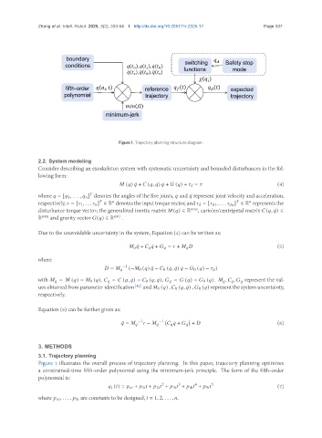
Figure 1. Trajectory planning structure diagram.

2.2. System modeling
Consider describing an exoskeleton system with systematic uncertainty and bounded disturbances in the fol-
lowing form:
( ) ¥ + ( , ¤) ¤ + ( ) + = (4)

where = [ 1 , . . . , ] denotes the angles of the five joints, ¤ and ¥ represent joint velocity and acceleration,

respectively, = [ 1 , . . . ] ∈ R denotestheinputtorquevector, and = [ 1 , . . . ] ∈ R representsthe
disturbance torque vector; the generalized inertia matrix ( ) ∈ R × , carioles/centripetal matrix ( , ¤) ∈

R × and gravity vector ( ) ∈ R ×1 .
Due to the unavoidable uncertainty in the system, Equation (4) can be written as:
¥ + ¤ + = + (5)

where
−1
= (− 0 ( ) ¥ − 0 ( , ¤ ) ¤ − 0 ( ) − )
with = ( ) − 0 ( ), = ( , ¤) − 0 ( , ¤), = ( ) − 0 ( ). , , represent the val-

ues obtained from parameter identification [42] and 0 ( ) , 0 ( , ¤) , 0 ( ) represent the system uncertainty,

respectively.
Equation (5) can be further given as:

−1 −1 (6)

¥ = − ¤ + +
3. METHODS

3.1. Trajectory planning
Figure 1 illustrates the overall process of trajectory planning. In this paper, trajectory planning optimizes
a constrained-time fifth-order polynomial using the minimum-jerk principle. The form of the fifth-order
polynomial is:
4
2
3
( ) = + 1 + 2 + 3 + 4 + 5 5 (7)
where , . . . , 5 are constants to be designed, = 1, 2, . . . , .