Page 55 - Read Online

Wang et al. Intell Robot 2023;3(3):479-94 I http://dx.doi.org/10.20517/ir.2023.26 Page 9 of 16

where = − , and Φ = Φ − Φ.
ˆ
ˆ
∗
∗
e
e
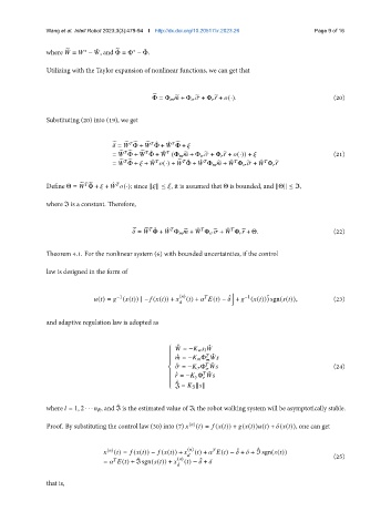
Utilizing with the Taylor expansion of nonlinear functions, we can get that
Φ = Φ e + Φ e + Φ e+ (·). (20)

e
Substituting (20) into (19), we get

e ˆ
= Φ + Φ + Φ +
e
e e
ˆ e
e ˆ
ˆ
= Φ + Φ + (Φ e + Φ e + Φ e + (·)) + (21)
e e
ˆ e ˆ ˆ ˆ ˆ
e e
= Φ + + (·) + Φ + Φ e + Φ e + Φ e
ˆ
Define Θ = Φ + + (·); since k k ≤ , it is assumed that Θ is bounded, and kΘk ≤ ℑ,
¯
e e
where ℑ is a constant. Therefore,

ˆ
ˆ
e ˆ
ˆ

= Φ + Φ e + Φ e + Φ e+ Θ. (22)

e
Theorem 4.1. For the nonlinear system (6) with bounded uncertainties, if the control
law is designed in the form of
k

−1
−1
ˆ
ˆ
( ) = ( ( )) | − ( ( )) + ( ) ( ) + ( ) − + ( ( ))) sgn( ( )), (23)

and adaptive regulation law is adopted as
 ¤
 ˆ ˆ
= −

 ˆ
 ˆ = − Φ

 ¤

 
ˆ
ˆ = − Φ (24)
¤

 ˆ
 ˆ = − Φ
 ¤


 ¤
 ˆ
= k k
 =
where = 1, 2 · · · , and ℑ is the estimated value of ℑ; the robot walking system will be asymptotically stable.
ˆ
Proof. By substituting the control law (30) into (7) ( ) ( ) = ( ( )) + ( ( )) ( ) + ( ( )), one can get

ˆ
ˆ
( ) ( ) = ( ( )) − ( ( )) + ( ) ( ) + ( ) − + + = sgn( ( ))
(25)

ˆ
ˆ
= ( ) + ℑ sgn( ( )) + ( ) ( ) − +

that is,