Page 57 - Read Online

Wang et al. Intell Robot 2023;3(3):479-94 I http://dx.doi.org/10.20517/ir.2023.26 Page 11 of 16

Table 1. Configuration parameters of robots
Torso Calf
Parameter Thigh length Calf length Trunk mass Thigh mass Calf length Thigh rotational inertia
length rotational inertia
Value unit 0.204 m 0.412 m 0.385 m 5.9 kg 13.2 kg 7.7 kg 0.56 2 0.28 2

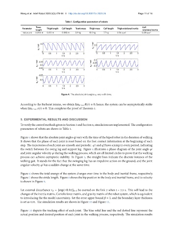
Figure 4. The absolute joint angles vary with time.

According to the Barbarat lemma, we obtain lim t→∞ ( ) = 0; hence, the system can be asymptotically stable
when lim →∞ ( ) = 0. This completes the proof of Theorem 1.

5. EXPERIMENTAL RESULTS AND DISCUSSION
ToverifythecontrolmethodsgiveninSection3andSection4,simulationsareimplemented. Theconfiguration
parameters of robots are shown in Table 1.

Figure 4 shows that the absolute joint angles qi vary with the time of the biped robot in the duration of walking.
It shows that the phase of each joint is reset based on the foot contact information at the beginning of each
step. The trajectories of each joint are smooth and periodic. 1 and 2 have a jump in every period, indicating
the switch between the swing leg and support leg. Figure 4 illustrates a phase diagram of the joint angle
and joint angular velocity during the walking process, which are all limited circles to prove that the walking
process can achieve asymptotic stability. In Figure 5, the straight lines indicate the discrete instance of the
walking gait. It stands for the fact that the swinging leg has an impulsive action on the ground, and the joint
angular velocity has a sudden change at the same time.

Figure 6 shows the total energy of the system changes over time in the body and inertial frame, respectively.
Figure 7 shows the stride length. Figure 8 shows the hip position in the body and inertial frame, and its velocity
is shown in Figure 9.

Let external disturbance = [exp(−0.1 )] 6×1 be exerted on the link 2 when t = 2.5 s. This will lead to the
changes of the inertia matrix, Coriolis force matrix, and gravity matrix of the robot system, which is equivalent
to introducing the the model uncertainty. Set the error upper bound = 1, and the boundary layer thickness
is set as 0.01. The simulation results are shown in Figure 10 and Figure 11.

Figure 10 depicts the tracking effect of each joint. The blue solid line and the red dotted line represent the
actual position and desired position of each joint in the walking process, respectively. The simulation results