Page 144 - Read Online

Page 429 Chen et al. Intell Robot 2023;3:420-35 https://dx.doi.org/10.20517/ir.2023.24

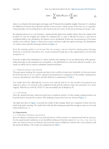
where (x, y) denotes the train input and target, and W denotes the trainable weights. Function l(·) calculates
the difference between the prediction and the correct answer, which is part of the loss. g(·) is a sparsity-
induced penalty on the scaling factors, and λ balances the two terms. In the sparse training, we let g(s) = |s|.

By using Equation (2) as a loss function, γ asymptotically approaches smaller values. Since the output is the
product of γ and the weights, the output of a channel with a γ near 0 will also be nearly 0, and since it
contributes little to the calculation, the channel can be eliminated. In this way, the parameters of the entire
model can be reduced. Figure 13 shows the accuracy and loss results after sparse learning. The distribution
of γ values before and after learning is shown in Figure 14.

From the training results, it can be seen that the accuracy took an initial dive during sparse learning.
However, it eventually returned to 80%. Losses increased sharply due to the regularization term but then
dropped to 1.6.

From the results of the distribution of γ before and after the training, we can see that because of the sparsity-
induced penalty on the scaling factors in Equation 1, the distribution of γ has been reduced to nearly 0. As a
result, we will be able to remove redundant channels and layers.

3.1.3. Reduction of layers and channels
Through sparse learning, the channels and layers that could be deleted were identified. In this experiment,
the threshold was set to 0.85, and the reduction was performed. A comparison of the number of parameters,
accuracy, and inference time before and after deletion is summarized in Table 2.

The results show that although the accuracy was reduced only by 8%, the number of parameters was
reduced to about 1.5% of those in the original network and the inference time was reduced to 40% of the
original. With the use of NCS2, YOLO V3 was successfully run in Raspberry Pi.

3.1.4. Fine-tuning
After the channel and layer reductions have been completed, another 300 fine-tuning training sessions can
be performed to increase the accuracy. The resulting accuracy and losses are shown in Figure 15.

The light blue lines in Figure 14 present the results of fine-tuning, which are compared to those from the
initial and sparse learning. The results show that the fine-tuning increased the average accuracy to 85% and
reduced the loss to 1.4.

3.2. Experiments
3.2.1 Verification of distance measurement
Since the distance measurement is an essential feature of this research, we experimented with its accuracy.
For the experimental conditions, we set six different distances from the camera (0.5 m, 1 m, 1.5 m, 2 m, 3 m,
and 4 m), used a person as an obstacle, and tested the extent of difference between the correct distance and
the measured distance. The results are summarized in Table 3.