Page 39 - Read Online

Chen et al. Complex Eng Syst 2023;3:8 I http://dx.doi.org/10.20517/ces.2022.50 Page 5 of 15

 (¤ − ) = + cos + + − + sin



  ¤
( + ) = + sin + + cos + +
(5)

 ¤ = + sin + − cos + ( − )
 2

 + + cos + − sin − ( + )
 2
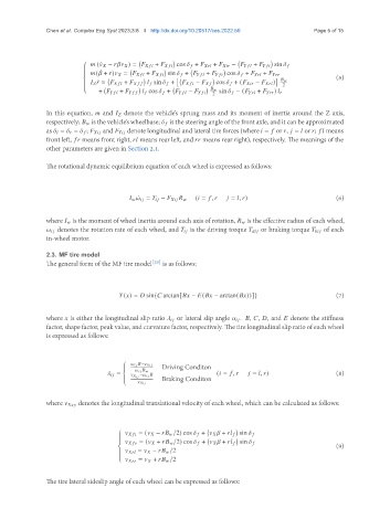
In this equation, and denote the vehicle’s sprung mass and its moment of inertia around the Z axis,
respectively; is the vehicle’s wheelbase; is the steering angle of the front axle, and it can be approximated
as = = ; and denote longitudinal and lateral tire forces (where = or , = or ; means
front left, means front right, means rear left, and means rear right), respectively. The meanings of the
other parameters are given in Section 2.1.
The rotational dynamic equilibrium equation of each wheel is expressed as follows:

¤ = − ( = , = , ) (6)

where is the moment of wheel inertia around each axis of rotation, is the effective radius of each wheel,
denotes the rotation rate of each wheel, and is the driving torque or braking torque of each
in-wheel motor.

2.3. MF tire model
The general form of the MF tire model [20] is as follows:

( ) = sin{ arctan[ − ( − arctan( ))]} (7)

where is either the longitudinal slip ratio or lateral slip angle . , , , and denote the stiffness
factor, shape factor, peak value, and curvature factor, respectively. The tire longitudinal slip ratio of each wheel
is expressed as follows:

 −
 Driving Conditon
 
= − ( = , = , ) (8)

 Braking Conditon



where denotes the longitudinal translational velocity of each wheel, which can be calculated as follows:

 = ( − /2) cos + + sin



  = ( + /2) cos + + sin
(9)
 = − /2



 = + /2
The tire lateral sideslip angle of each wheel can be expressed as follows: