Page 42 - Read Online
P. 42
Page 8 of 15 Chen et al. Complex Eng Syst 2023;3:8 I http://dx.doi.org/10.20517/ces.2022.50
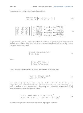
The partial derivative in Eq. (15) can be calculated as follows:
h i
¤ ¤ ¤
= (17a)
¤ ¤ ¤
− ( /2+ ) + /2
2 − /2 2
( − /2) ( − /2)
( /2− ) − /2
2 + /2 2
= ( + /2) ( + /2) (17b)
− ( /2− ) − + /2
2 − /2 2
( − /2) ( − /2)
( /2+ ) − − /2
2 + /2 2
( + /2) ( + /2)
The parameters and can be obtained from the MF tire model by using Eq. (12). The parameters in
matrix , which is detailed in Eqs. (16) and (17), can be expressed using the results of the -th step. Then, Eq.
(15) can be discretized as follows:
( + 1) = ( ) ( ) + ( ) ( )
(18)
( ) = ( )
where
(
( ) = ( ) ≈ ( ) +
¯
( ) = · ≈
0
The discrete linear equation for MPC control can be rewritten in the following form:
Δ ( + 1) = ( )Δ ( ) + Δ ( )
(19)
( ) = ( − 1) + Δ ( )
where Δ ( ) = ( ) − ( − 1), and Δ ( ) = ( ) − ( − 1). The predictive time domain of this system is
composed of steps, control time domain of this system is composed of steps, and the relationship ≤
holds. In this work, and are set to 8 and 3, respectively. The -step control input vector and -step
predictive output vector can be expressed as follows:
(
Δ ( ) = Δ ( ) Δ ( + 1) · · · Δ ( + − 1)
(20)
( ) = ( + 1) ( + 2) · · · ( + ) · · · ( + )
Therefore, the output vector of each future predictive steps is given as follows:

