Page 68 - Read Online

Page 12 of 20 Huang et al. Complex Eng Syst 2023;3:2 I http://dx.doi.org/10.20517/ces.2022.43

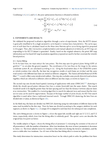
Combining (19), (21), and (23), the pose optimization function is obtained as follows:

Õ

T
ˆ
= arg min ( −1 , , ) Ω ( , , )

Õ
T
+ ( , , ) Ω ( , , )
(24)

Õ
( ) T
+ ( − ) ( − )
2

6. EXPERIMENTS AND RESULTS
We validated the proposed localization algorithm through a series of experiments. First, the KITTI dataset
is gradually simplified to fit a single parametric curve based on various lane characteristics. The curve equa-
tion of each lane line is calculated based on the three-time Hermite spline curve fitting algorithm proposed
in this paper. Then, after intersection complementation and manual adjustment of elements, an HD map cor-
responding to the KITTI dataset is generated. Finally, based on the original odometry, the priori HD map
information and the fused HD map localization algorithm proposed are used to further constrain the vehicle’s
lateral position.
6.1. Curve fitting
To fit the lane lines, we must extract the lane points. The first step uses the ground plane fitting (GPF) al-
gorithm [30] to calculate the ground equation. The coordinates of the lane lines on the image in the camera
coordinate system c are calculated according to (5). Using the localization data of the GNSS/INS system
as vehicle position true value b, the lane line recognition results of each frame are stitched and the same
road section with different lane lines are stored as different categories. The StatisticalOutlierRemoval (SOR)
filter [38] is used to filter some misdetected outliers. This step also excludes some poorly detected road sections
together, which are reflected as different colors in different lane line maps, as shown in Figure 5(a).

The second step uses density-based spatial clustering of applications with noise (DBSCAN) [39] clustering to
divide the closely spaced points (distance less than a certain threshold) into the same cluster. This search
threshold needs to be slightly greater than the lane spacing and less than the distance between adjacent lanes
at an intersection. This enables the clustering algorithm to search for adjacent lanes and ensure that the inter-
section area can be used for segmentation. Because of the large number of point clouds, the KD-Tree search
algorithm is used rather than a traditional traversal search. Through DBSCAN clustering, the lane lines are
divided into 19 areas, as shown in Figure 5(b).

In the third step, the lanes are divided via DBSCAN clustering using the information of different lanes in the
same road recorded in the first step. Then the lanes are divided according to the category attribute for each
segment, as shown in Figure 5(c). A unique ID is assigned to each lane here for subsequent lane completion.

The curve fitting process is shown in Figure 6, where the upper left, middle and right are X-Y, X-Z, and Y-Z
views, respectively, which show that the fitting effect is relatively good. The spatial curve can describe the
original lane line point set better.

The middle subplot of Figure 6 shows the fitting effect of parameter t, indicating the variation of the error of
all parameters i with the number of iterations. After four iterations, the error of most parameters i decreases
to below 1.0. The lower subplot shows the variation of the total error during the iterative calculation, and the
error is stable after two iterations. The 3D view of this lane line fitting effect is shown in Figure 7.

This study determines the intersection connection based on the vehicle path to solve the problem that there