Page 63 - Read Online

Huang et al. Complex Eng Syst 2023;3:2 I http://dx.doi.org/10.20517/ces.2022.43 Page 7 of 20

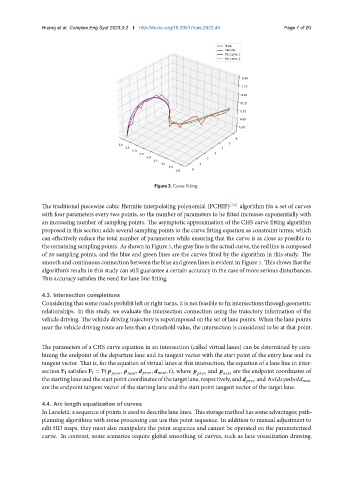
Figure 3. Curve fitting.

The traditional piecewise cubic Hermite interpolating polynomial (PCHIP) [32] algorithm fits a set of curves
with four parameters every two points, so the number of parameters to be fitted increases exponentially with
an increasing number of sampling points. The asymptotic approximation of the CHS curve fitting algorithm
proposed in this section adds several sampling points to the curve fitting equation as constraint terms, which
can effectively reduce the total number of parameters while ensuring that the curve is as close as possible to
the remaining sampling points. As shown in Figure 3, the gray line is the actual curve, the red line is composed
of 20 sampling points, and the blue and green lines are the curves fitted by the algorithm in this study. The
smooth and continuous connection between the blue and green lines is evident in Figure 3. This shows that the
algorithm’s results in this study can still guarantee a certain accuracy in the case of more serious disturbances.
This accuracy satisfies the need for lane line fitting.

4.3. Intersection completions
Considering that some roads prohibit left or right turns, it is not feasible to fix intersections through geometric
relationships. In this study, we evaluate the intersection connection using the trajectory information of the
vehicle driving. The vehicle driving trajectory is superimposed on the set of lane points. When the lane points
near the vehicle driving route are less than a threshold value, the intersection is considered to be at that point.

The parameters of a CHS curve equation in an intersection (called virtual lanes) can be determined by com-
bining the endpoint of the departure lane and its tangent vector with the start point of the entry lane and its
tangent vector. That is, for the equation of virtual lanes at this intersection, the equation of a lane line in inter-
section F I satisfies F I = F( , , , , ), where and are the endpoint coordinates of
thestartinglaneandthestartpointcoordinatesofthetargetlane, respectively, and and
are the endpoint tangent vector of the starting lane and the start point tangent vector of the target lane.

4.4. Arc length equalization of curves
In Lanelet2, a sequence of points is used to describe lane lines. This storage method has some advantages; path-
planning algorithms with some processing can use this point sequence. In addition to manual adjustment to
edit HD maps, they must also manipulate the point sequence and cannot be operated on the parameterized
curve. In contrast, some scenarios require global smoothing of curves, such as lane visualization drawing.