Page 61 - Read Online

Huang et al. Complex Eng Syst 2023;3:2 I http://dx.doi.org/10.20517/ces.2022.43 Page 5 of 20

4.1. Inverse perspective mapping with ground equation
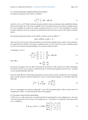
The projection equation of the camera is as follows:

uv
c = c = cb b (1)
1
where c = [ c , c , c ] isthecoordinatesofapointunderthecameracoordinatesystem,and istheintrinsic
T
matrix of the camera. c is the -axis coordinate of the actual ground point in the camera coordinate system.
b is the coordinates of a point in the vehicle coordinate system, uv = [ , ] is the coordinates of a point in
T
the pixel coordinate system, cb represents transformation matrix from the camera to the vehicle coordinate
system.

We calculate the ground equations in the LiDAR coordinate system as follows [30] :
T
T
T
l = lc c = c = − (2)
l l c
where l is the vector normal to the ground plane in the LiDAR coordinate system, and lc is the transforma-
tion matrix from the LiDAR to the camera coordinate system. 1 is the point in the radar coordinate system.
c is the vector normal to the ground plane in the camera coordinate system.
Combining (1) and (2),
 
 0 0 
 uv 
 
   0 0 
 1  (3)
 =   c = cb b
  0 0 1
 0   0  
 
 
 
where is:

0
= (4)
T
c
The physical meaning of is the offset of the plane in the direction of the normal vector (after normalizing
the normal vector ). In the camera coordinate system, in the ground equation cannot be zero. Therefore,
it can be assumed that is full rank.
Since the matrix varies with the ground equation, its inverse matrix must be calculated for each subsequent
frame, and the program overhead is significant. From the chunk matrix property, we can further obtain the
following:
−1  uv 
1 0  
c = −1 T −1  1  (5)
− −1    
c
 0 
From (5), the program only needs to compute once in the initialization phase. Then, it is just a matter of
−1
computing and in each subsequent frame of the program.
−1
′T
4.2. Piecewise cubic hermite spline fitting
A CHS curve is a cubic polynomial curve determined by the starting point 0, the ending point 1, the slope
of the starting point 0, and the slope of the ending point 1. The equation of a parametric cubic polynomial
curve is defined as:
T
2
   1 − 3 + 2 3
   
 
  +1  3 − 2 3 
2
F ( , +1 , , +1 , ) = =    2 3   (6)

   − 2 + 
   2 3 
 +1   − + 
   