Page 67 - Read Online

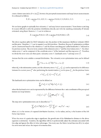
Huang et al. Complex Eng Syst 2023;3:2 I http://dx.doi.org/10.20517/ces.2022.43 Page 11 of 20

between the perceptual measurements and map feature measurements.
create a feature association = { } =1
It is obtained as follows:
ˆ ˆ
, = arg max ( , | , ) = arg max ( | , , ) ( | , , ) (17)
, ,

We use factor graphs to optimally fuse odometry and map feature measurements from feature matching.

It is more difficult to solve the posterior distribution directly, and with the matching relationship already
ˆ
estimated, using Bayes’ theorem, (17) can be written as
ˆ ˆ ˆ
= arg max ( | , , ) = arg max ( ) ( | , , ) (18)

The above equation splits the MAP estimation into the product of the maximum likelihood estimate (MLE)
and the prior. Therefore, (17) can be equated to an MLE problem. Therefore, the pose optimization problem

can be constructed based on the odometry and the feature matching pair (called landmarks) obtained in

the previous section. The error term consists of the odometry error and the observation error . The obser-

vation error can be composed of the coordinate error of the landmark and the map error . Therefore,

we divide the error term into three parts: odometry error , landmark error and map error .

Assume that the noise satisfies a normal distribution. The odometry error optimization term can be defined
as:
Õ
T
( −1 , , ) Ω ( −1 , , ) (19)

where Ω is the information matrix, and the odometry error ( , , ) can be expressed as the difference
−1

between the current pose T after performing the transformation on the pose for the previous frame:
−1

( , , ) = T (20)
−1 −1
The landmark error optimization term can be defined as:
Õ

( , , ) Ω ( , , ) (21)

wherethelandmarkerrorcanberepresentedbythedifferencebetweenthe -axiscoordinatesoftheperceptual
features and map features:

T 1 T
( , , ) = cb − (22)

0
The map error optimization term can be described as [37] :
Õ T ( ) Õ T
( ) Ω ( ) = 2 ( − ) ( − ) (23)

where ( ) is the inverse-chi-squared distribution function, is the radius, and is the location of the th
frame map feature.
When the error of a particular edge is significant, the growth rate of the Mahalanobis distance in the above
equation is substantial. Therefore, the algorithm will try to preferentially adjust the estimates associated with
this edge and ignore the effect of other advantages. This study uses the Huber kernel function ( ) to adjust
the error term and reduce the impact of erroneous data.