Page 16 - Read Online

Page 12 of 15 Fan et al. Complex Eng Syst 2023;3:5 I http://dx.doi.org/10.20517/ces.2023.04

0.2 0.2
0.15 0.15
Weights of the critic network 1 0.05 0 Weights of the critic network 2 0.05 0
0.1
0.1

-0.05

-0.1 -0.05
-0.1
-0.15 -0.15
0 50 100 150 200 250 300 350 400 450 500 550 600 0 50 100 150 200 250 300 350 400 450 500 550 600
Time (s) Time (s)
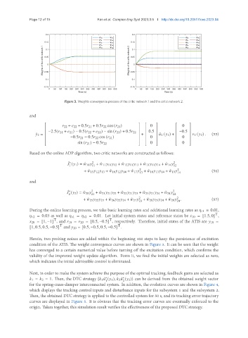
Figure 3. Weights convergence process of the critic network 1 and the critic network 2.

and

 22 + 22 + 0.5 21 + 0.5 22 cos ( 21 )   0   0 
     
     
 −2.5( 21 + 21 ) − 0.5( 22 + 22 ) − sin ( 21 ) + 0.5 22   0.5   −0.5  (55)
¤ 2 =   +   ¯ 2 ( 2 ) +   2 ( 2 ) .
 −0.5 21 − 0.5 22 cos ( 21 )   0   0 
     
 sin ( 21 ) − 0.5 22   0   0 
     
Based on the online ADP algorithm, two critic networks are constructed as follows:
ˆ
∗
( 1 ) = ˆ 10 2 + ˆ 11 11 12 + ˆ 12 11 13 + ˆ 13 11 14 + ˆ 14 2
1 11 12
+ ˆ 15 12 13 + ˆ 16 12 14 + ˆ 17 2 + ˆ 18 13 14 + ˆ 19 2 (56)
13 14
and

ˆ
( 2 ) = ˆ 20 2 + ˆ 21 21 22 + ˆ 22 21 23 + ˆ 23 21 24 + ˆ 24 2
∗
2 21 22
2
+ ˆ 25 22 23 + ˆ 26 22 24 + ˆ 27 2 + ˆ 28 23 24 + ˆ 29 . (57)
23 24
During the online learning process, we take basic learning rates and additional learning rates as 1 = 0.01,
T
2 = 0.03 as well as 1 = 2 = 0.01. Let initial system states and reference states be 10 = [1.5, 0] ,
T T
20 = [1, −1] , and 10 = 20 = [0.5, −0.5] , respectively. Therefore, initial states of the ATIS are 10 =
T
T
[1, 0.5, 0.5, −0.5] and 20 = [0.5, −0.5, 0.5, −0.5] .
Herein, two probing noises are added within the beginning 400 steps to keep the persistence of excitation
condition of the ATIS. The weight convergence curves are shown in Figure 3. It can be seen that the weight
has converged to a certain numerical value before turning off the excitation condition, which confirms the
validity of the improved weight update algorithm. Form it, we find the initial weights are selected as zero,
which indicates the initial admissible control is eliminated.

Next, in order to make the system achieve the purpose of the optimal tracking, feedback gains are selected as
1 = 2 = 1. Then, the DTC strategy { 1 ˆ ( 1 ), 2 ˆ ( 2 )} can be derived from the obtained weight vector
∗
∗
2
1
for the spring-mass-damper interconnected system. In addition, the evolution curves are shown in Figure 4,
which displays the tracking control inputs and disturbance inputs for the subsystem 1 and the subsystem 2.
Then, the obtained DTC strategy is applied to the controlled system for 50 s, and its tracking error trajectory
curves are displayed in Figure 5. It is obvious that the tracking error curves are eventually enforced to the
origin. Taken together, this simulation result verifies the effectiveness of the proposed DTC strategy.