Page 15 - Read Online

Fan et al. Complex Eng Syst 2023;3:5 I http://dx.doi.org/10.20517/ces.2023.04 Page 11 of 15

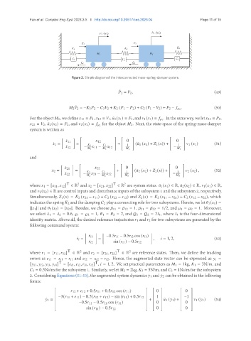
P 1 9 1 P 2 9 2

F 1 F 2
K 3
K 1 K 2
M 1 M 2
C 1 C 2 C 3
f ȝ1 f ȝ2

Figure 2. Simple diagram of the interconnected mass–spring–damper system.

2 = 2 , (49)
¤

¤ . (50)
2 2 = − 3 2 − 3 2 + 2 ( 1 − 2 ) + 2 ( 1 − 2 ) + 2 − 2
. Inthesameway, welet 21 = 2,
Fortheobject 1, wedefine 11 = 1, 12 = 1, ¯ 1 ( 1 ) = 1, and 1 ( 1 ) = 1
for the object 2. Next, the state-space of the spring-mass-damper
22 = 2, ¯ 2 ( 2 ) = 2, and 2 ( 2 ) = 2
system is written as
" # " # " #

¤ 11 12 0 0
¤ 1 = = 1 1 + 1 ( ¯ 1 ( 1 ) + 1 ( )) + 1 1 ( 1 ) (51)
¤ 12 − 11 − 12 −
1 1 1 1
and
" # " # " #

¤ 21 22 0 0
¤ 2 = = 3 3 + 1 ( ¯ 2 ( 2 ) + 2 ( )) + 1 2 ( 2 ) , (52)
¤ 22 − 21 − 22 −
2 2 2 2
T 2 T 2
where 1 = [ 11 , 12 ] ∈ R and 2 = [ 21 , 22 ] ∈ R are system states. ¯ 1 ( 1 ) ∈ R, ¯ 2 ( 2 ) ∈ R, 1 ( 1 ) ∈ R,
and 2 ( 2 ) ∈ R are control inputs and disturbance inputs of the subsystem 1 and the subsystem 2, respectively.
Simultaneously, 1 ( ) = 2 ( 21 − 11 ) + 2 ( 22 − 12 ) and 2 ( ) = 2 ( 11 − 21 ) + 2 ( 12 − 22 ), which

indicates the spring 2 and the damping 2 play a connecting role for two subsystems. Herein, we let 1 ( 1 ) =
|| 1 || and 2 ( 2 ) = | 22 |. Besides, we choose 11 = 12 = 1, 21 = 22 = 1/2, and 1 = 2 = 1. Moreover,
we select 1 = 2 = 0.6, 1 = 2 = 1, 1 = 2 = 2, and 1 = 2 = 2 4, where 4 is the four-dimensional
identity matrix. Above all, the desired reference trajectories 1 and 2 for two subsystems are generated by the
following command system:

¤ 1 −0.5 1 − 0.5 2 cos ( 1 )
¤ = = , = 1, 2, (53)
¤ 2 sin ( 1 ) − 0.5 2
T 2 T 2
where 1 = [ 11 , 12 ] ∈ R and 2 = [ 21 , 22 ] ∈ R are reference states. Then, we define the tracking
errors as 1 = 1 − 1 and 2 = 2 − 2. Hence, the augmented state vector can be expressed as =
T T
[ 1 , 2 , 3 , 4 ] = [ 1 , 2 , 1 , 2 ] , = 1, 2. We set practical parameters as 1 = 1kg, 1 = 3N/m, and
1 = 0.5Ns/m for the subsystem 1. Similarly, we let 2 = 2kg, 3 = 5N/m, and 3 = 1Ns/m for the subsystem
2. Considering Equations (51-53), the augmented system dynamics ¤ 1 and ¤ 2 can be obtained in the following
forms:

 12 + 12 + 0.5 11 + 0.5 12 cos ( 11 )   0   0 
     
     
 −3( 11 + 11 ) − 0.5( 12 + 12 ) − sin ( 11 ) + 0.5 12   1   −1  (54)
¤ 1 =   +   ¯ 1 ( 1 ) +   1 ( 1 )
 −0.5 11 − 0.5 12 cos ( 11 )   0   0 
     
 sin ( 11 ) − 0.5 12   0   0 
     