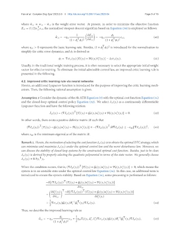
Page 13 - Read Online

Fan et al. Complex Eng Syst 2023;3:5 I http://dx.doi.org/10.20517/ces.2023.04 Page 9 of 15

where ˜ = − ˆ is the weight error vector. At present, in order to minimize the objective function
T
= (1/2) , the normalised steepest descent algorithm based on Equation (38) is employed as follows:

1
¤ ˆ = − = − , (40)
T T 2
(1 + ) 2 ˆ (1 + )

T
2
where > 0 represents the basic learning rate. Besides, (1 + ) is introduced for the normalization to

simplify the critic error dynamics, and is derived as
∗
= ∇ ( )[F ( ) + H ( ) ˆ ( )] − ( ). (41)

Usually, in the traditional weight training process, it is often necessary to select the appropriate initial weight
vector for effective training. To eliminate the initial admissible control law, an improved critic learning rule is
presented in the following.
4.2. Improved critic learning rule via neural networks
Herein, an additional Lyapunov function is introduced for the purpose of improving the critic learning mech-
anism. Then, the following rational assumption is given.

Assumption1Considerthedynamicofthe thATISEquation(9) withtheoptimalcostfunctionEquation(14)
and the closed-loop optimal control policy Equation (32). We select ( ) as a continuously differentiable
Lyapunov function and have the following relation:

T
∗
( ) = (∇ ( )) [F ( ) + G ( ) ( ) + H ( ) ( )] < 0. (42)
∗
¤

In other words, there exists a positive definite matrix ℬ such that
T
T
2
(∇ ( )) [F ( ) + G ( ) ( ) + H ( ) ( )] = −(∇ ( )) ℬ∇ ( ) ≤ − k∇ ( )k , (43)
∗
∗

where is the minimum eigenvalue of the matrix ℬ.
Remark2. Herein,themotivationofselectingthecostfunction ( ) istoobtaintheoptimalDTCstrategy, which
can minimize and maximize ( ) under the optimal control law and the worst disturbance law. Moreover, we
can discuss the stability of closed-loop systems by the constructed optimal cost function. Besides, just to be clear,
( ) is derived by properly selecting the quadratic polynomial in terms of the state vector. We generally choose
T
( ) = 0.5 .
T
When the condition occurs, that is, (∇ ( )) [F ( ) + G ( ) ( ) + H ( ) ( )] > 0, which means the
∗
∗

system is in an unstable state under the optimal control law Equation (36). In this case, an additional term is
introduced to ensure the system stability. Based on Equation (36), some processing is performed as follows:
T
∗
∗
− [(∇ ( )) (F ( ) + G ( ) ( ) + H ( ) ( ))]

ˆ
∗ T T ∗ ∗
ˆ ( ) − [(∇ ( )) (F ( ) + G ( ) ( ) + H ( ) ( ))]

=
∗
ˆ ˆ ( )

1 −1 T
= ∇ ( )G ( ) G ( )∇ ( ). (44)

2
Thus, we describe the improved learning rule as
1 −1 T
∗
∗
¤ ˆ = − + Π ( , ˆ , ˆ )∇ ( )G ( ) G ( )∇ ( ), (45)

T
(1 + ) 2 2