Page 11 - Read Online

Fan et al. Complex Eng Syst 2023;3:5 I http://dx.doi.org/10.20517/ces.2023.04 Page 7 of 15

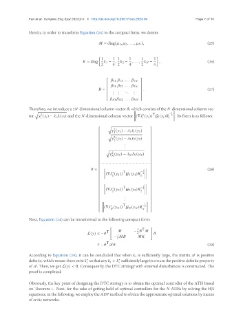
Herein, in order to transform Equation (24) to the compact form, we denote

= diag{ 1 , 2 , . . . , }, (25)

1 1 1 1 1 1
= diag 1 − , 2 − , . . . , − , (26)
2 4 2 4 2 4

 11 12 . . . 1 
 
 21 22 . . . 2 
  (27)
=  . . . . . . . .  .
 . . . . 
 
 
 1 2 . . . 
Therefore, we introduce a 2 -dimensional column vector , which consists of the -dimensional column vec-
q
1

T
−
tor ( ) − ( ) and the -dimensional column vector (∇ ( )) G ( )
. Its form is as follows:
2
∗

2

q
 2 
 ( 1 ) − 1 1 ( 1 ) 
1
 q 
 2 
 ( 2 ) − 2 2 ( 2 ) 
2
 
 . . 
 . 
 
q
 2 
 ( ) − ( ) 

 
 
 
 
 
= 

 (28)

T − 1

∗

(∇ ( 1 )) G 1 ( 1 ) 2


1 1

 
 




T − 1

∗

(∇ ( 2 )) G 2 ( 2 ) 2


2 2

 
 . . 
 . 




T − 1

(∇ ( )) G ( )

∗ 2




 
Next, Equation (24) can be transformed to the following compact form:
" 1 T #
L( ) ≤ − T −
¤
2
1
−
2
T
≜ − . (29)
According to Equation (29), it can be concluded that when is sufficiently large, the matrix is positive
definite, whichmeansthereexist sothatany > sufficientlylargetoensurethepositivedefiniteproperty
∗
∗

of . Then, we get L( ) < 0. Consequently, the DTC strategy with external disturbances is constructed. The
¤
proof is completed.
Obviously, the key point of designing the DTC strategy is to obtain the optimal controller of the ATIS based
on Theorem 1. Next, for the sake of getting hold of optimal controllers for the ATISs by solving the HJI
equations, in the following, we employ the ADP method to obtain the approximate optimal solutions by means
of critic networks.