Page 12 - Read Online

Page 8 of 15 Fan et al. Complex Eng Syst 2023;3:5 I http://dx.doi.org/10.20517/ces.2023.04

4. OPTIMAL DTC DESIGN VIA NEURAL NETWORKS
4.1. Implementation procedure via neural networks
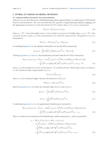
Inthissection,weshowtheprocessoffindingtheapproximateoptimalsolutionbyemployingtheADPmethod
based on neural networks. The critic networks have the capability of approximating nonlinear mapping, and
the approximate cost function can be derived for the DTC system. Hence, ( ) can be expressed as
∗

T
∗
( ) = ( ) + ( ), (30)

where ∈ R is the ideal weight vector, is the number of neurons in the hidden layer, ( ) ∈ R is the

activation function, and ( ) is the reconstruction error of the th neural network. The gradient of ( ) is
∗

formulated as
T
∇ ( ) = (∇ ( )) + ∇ ( ), (31)
∗

Considering Equation (16), the optimal control policy for the th ATIS is replaced by
1 −1 T T
( ) = − G ( ) (∇ ( )) + ∇ ( ) . (32)
∗

2
Utilizing Equations (31) and (32), the Hamiltonian associated with the th ATIS is obtained as
2 T T
( , ( ), ) = ( ) − ( ( )) + (∇ ( ))[F ( ) + H ( ) ( )]

1 T −1 T T
− ∇ ( )G ( ) G ( )(∇ ( )) + ℎ = 0, (33)

4
where ℎ is the residual error of the neural network. To avoid the unknown ideal weight vector, we construct
critic neural networks to approximate ( ) as
∗

T
ˆ
∗
( ) = ˆ ( ), (34)

where ˆ is the estimated weight. Likewise, the derivative of ( ) is
ˆ ∗

T
ˆ
∇ ( ) = (∇ ( )) ˆ . (35)
∗

Based on Equation (35), we obtain the estimated value of ( ) and ( ) as
∗
∗

1 −1 T T
ˆ ( ) = − G ( )(∇ ( )) ˆ , (36)
∗

2
1 T T
∗
ˆ ( ) = H ( )(∇ ( )) ˆ . (37)

2 2

Considering Equations (34-36), the approximate Hamiltonian is expressed as
ˆ ∗ 2 T T ∗
( , ˆ ( ), ˆ ) = ( ) − ( ˆ ( )) + ˆ (∇ ( ))[F ( ) + H ( ) ˆ ( )]

1 T −1 T T
− ∇ ( )G ( ) G ( )(∇ ( )) ˆ = . (38)
ˆ

4
Then, we obtain an error function of the Hamiltonian, which is denoted as and is expressed by
ˆ ∗
= ( , ˆ ( ), ˆ ) − ( , ( ), )

T T
= ( ˜ ( )) − ˜ (∇ ( ))[F ( ) + H ( ) ( )]

1 T −1 T T
˜
− ∇ ( )G ( ) G ( )(∇ ( )) ˜

4
1 T −1 T T
+ ∇ ( )G ( ) G ( )(∇ ( )) ˜ − ℎ , (39)

2