Page 76 - 2417

Salmerón et al. Carbon Footprints 2026, 5, 17 Page 7 of 26

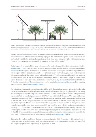
Figure 2. Representation of a 2-axis tracking agrivoltaic system integrated into an olive grove. The system configuration is defined by the
distance between panel rows (d), the olive tree height (h t ), and the panel installation height (h p ). The tracking mechanism allows panel
movement on both North-South and East-West axes to optimize solar capture while minimizing shading on the crop.

spacing, and orientation being critical for balancing energy generation with the preservation of agricultural
productivity [30-32,55-57] . The literature consistently highlights that intensive olive groves on low-slope terrain are
particularly suitable for AVS implementation, as their structured layout provides sufficient inter-row
clearance for photovoltaic structures without impeding mechanized harvesting [31,32,58] .

Building on this, a suitability analysis was performed using gridded datasets as described in
Supplementary Text 2. Grid cells were filtered to identify the most suitable areas for AVS deployment based
on criteria chosen to proxy intensive olive cultivation. The analysis selected grid cells with a slope of less than
5% to represent low-slope terrain and, to identify intensive cultivation, grid cells with irrigation
infrastructure, a key differentiator from traditional cultivations . A density threshold requiring at least 80%
[19]
olives within the grid cell was further applied to secure high density of installations. Together, these criteria
isolate the intensive olive groves that are best suited for AVS, resulting in a final estimated area of 76,186 ha.
A visual representation of the selection criteria can be seen in Supplementary Figure 3, and the resulting
suitable areas for AVS in Supplementary Figure 4.

For estimating the electricity generation potential for AVS, the suitable areas were intersected with a solar
resource map from Solargis [Supplementary Figure 5] to determine the specific photovoltaic electricity
production potential (kWh kWp ) for each location . To translate this potential into a total generation
-1
[28]
capacity (MW), an installed power density (MW ha ) was established. European AVS reports identify a
-1
range from 0.2 to 0.9 MW ha -1[59,60] . To prioritize the agricultural use of the land, a conservative baseline value
of 0.4 MW ha (with a range of ±0.2 MW ha considered in the Monte Carlo uncertainty analysis) was
-1
-1
adopted to represent differences in PV intensity. This aligns with literature on AVS in olive groves, where
installed potentials range from 0.29 to 0.43 MW ha , as olive trees exhibit moderate sensitivity to
-1
shading [30,31,60,61] . Based on a literature review of different AVS designs [Supplementary Table 8], the
technology selected for this study is a 2-axis tracking system [Figure 2], as its dynamic movement on both
N-S and E-W axes maximizes solar radiation capture while ensuring the minimum interference with the
olive trees [33,55] . The specifications of the system are available on Supplementary Table 9.

This suitability analysis established the total hectares available for AVS. From this, we defined two levels of
implementation: a low deployment level, representing an application to 50% of the suitable area identified,
and a high deployment level, representing an application of 100%.