Page 56 - 2417

François et al. Carbon Footprints 2026, 5, 22 Page 9 of 22

the ratio between the dynamic and the static characterization factors, for each type of GHG, at a given
moment of emission t and for a given integration time T. Given that CO , CH and N O represent the
4
2
i
2
overwhelming share of climate‑forcing emissions globally, the differing behaviors of α and β are particularly
relevant for these three gases. This is demonstrated in the case study in Section 4 and documented in
Supplementary Part 3 and Supplementary Figures 1-4.
Delay factor α for the global warming potential characterization factor
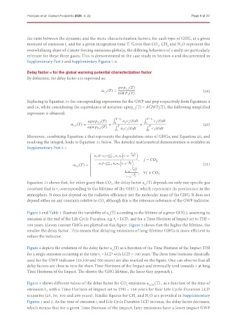
By definition, the delay factor α is expressed as:

6F? 8, 9 ())
0 8, 9 ()) = (19)
,% 9 ())
Replacing in Equation 19 the corresponding expressions for the GWP and gwp respectively from Equations 4
and 16, while considering the equivalence of notation agwp (T) = AGWP (T), the following simplified
o,j
j
expression is obtained:
∫ )−C 8 ∫ )−C 8
06F? 8, 9 ()) 0 9 2 9 (C)3C 2 9 (C)3C
0
0
0 8, 9 ()) = = ∫ = ∫ (20)
06F? 0, 9 ()) ) 0 9 2 9 (C)3C ) 2 9 (C)3C
0 0
Moreover, combining Equation 2 that represents the degradation rates of GHGs, and Equation 20, and
resolving the integral, leads to Equation 21 below. The detailed mathematical demonstration is available in
Supplementary Part 3.1.

)−C 8
 Í 3 − g =
 1 0 ()−C 8 )+
 ==1 1 = g = 1−4

 ,
 9 = $ 2
)
  1 0 )+ Í 3 − g = (21)
U 8, 9 ()) = ==1 1 = g = 1−4
 )−C 8

 1−4 − g 9

 ) , ∀9 ≠ $ 2

− g 9
 1−4
Equation 21 shows that, for other gases than CO , the delay factor α (T) depends on only one specific gas
i,j
2
constant that is τ corresponding to the lifetime of the GHG j, which represents its persistence in the
j
atmosphere. It does not depend on the radiative efficiency nor the molecular mass of the GHG. It does not
depend either on any constants relative to CO although this is the reference substance of the GWP indicator.
2
Figure 3 and Table 1 illustrate the variability of α (T) according to the lifetime of a given GHG j, assuming its
i,j
emission at the end of the Life Cycle Duration, e.g. t = LCD, and for a Time Horizon of Impact set to THI =
i
100 years. Eleven current GHGs are plotted on this figure. Figure 3 shows that the higher the lifetime, the
smaller the delay factor. This means that delaying emissions of long-lifetime GHGs is more efficient to
reduce the indicator.
Figure 4 depicts the evolution of the delay factor α (T) as a function of the Time Horizon of the Impact THI
i,j
for a single emission occurring at the time t = LCD with LCD = 100 years. The three time horizons classically
i
used for the GWP indicator (20,100 and 500 years) are also marked on the figure. One can observe that all
delay factors are close to zero for short Time Horizons of the Impact and eventually tend towards 1 at long
Time Horizons of the Impact. The shorter the GHG lifetime, the faster they approach 1.
Figure 5 shows different values of the delay factor for CO emissions α i,CO2 (T) , as a function of the time of
2
emission t , with a Time Horizon of Impact set to THI = 100 years for four Life Cycle Duration LCD
i
scenarios (25, 50, 100 and 200 years). Similar figures for CH and N O are provided in Supplementary
2
4
Figures 1 and 2. As the time of emission t and Life Cycle Duration LCD increase, the delay factor decreases,
i
which means that for a given Time Horizon of the Impact, later emissions have a lower impact GWP