


Page 54 - 2417
P. 54
François et al. Carbon Footprints 2026, 5, 22                                     Page 7 of 22


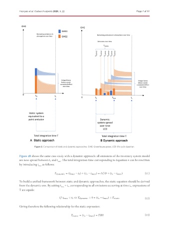
                         Figure 2. Comparison of static and dynamic approaches. GHG: Greenhouse gases; LCD: life cycle duration.

               Figure 2B shows the same case study with a dynamic approach: all emissions of the inventory system model
               are now spread between t 0 and t . The total integration time corresponding to Equation 9 can be rewritten
                                          max
               by introducing t  as follows:
                            max


                                        ) 3H=0<82 = (C <0G − C 0 ) + (C G − C <0G ) = !   + (C G − C <0G )  (11)
               To build a unified framework between static and dynamic approaches, the static equation should be derived
               from the dynamic one. By setting t  = t 0, corresponding to all emissions occurring at time t 0, expressions of
                                            max
               T are equals:


                                                                                                       (12)
                                           8 5 C <0G = C 0 ⇔ ) 3H=0<82 = 0 + (C G − C <0G ) = ) BC0C82
               Giving therefore the following relationship for the static expression:


                                                   ) BC0C82 = (C G − C <0G ) = )                       (13)

