Page 124 - Read Online

Page 6 of 15 Cheng et al. Soft Sci. 2026, 6, 36

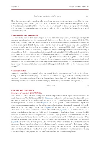
Production Rate (m/h) = (πd) × ω × 60 (1)

Here, d represents the diameter of the take-up roll, and ω represents the rotational speed. Therefore, the

cortisol-sensing yarn collection speed is 7.2 m/h. The process was carried out under a temperature of 30 ±
5 °C and a relative humidity of 50% ± 10%. The same conductive carbon thread was repeatedly subjected to
this conjugate electrospinning process for 1 to 4 cycles to achieve a well-defined coaxially structured
cortisol-sensing yarn.

Characterization and measurement
The surface and cross-section morphologies, as well as elemental compositions, were analyzed using field
emission scanning electron microscopy coupled with energy dispersive spectroscopy (FESEM-EDS,
Gemini500). The fine microstructure of NiHCF-MIP NCs was examined by high-resolution transmission
electron microscopy (HRTEM, Thermo Fisher Scientific Talos F200X G2). Chemical composition and crystal
structure were characterized by Fourier transform infrared spectroscopy (FTIR, Nicolet 5700) and X-ray
diffraction (XRD, Bruker D8 A8 Advance), respectively. Electrochemical performance was assessed using a
standard three-electrode system and an electrochemical workstation (CHI760E). The cortisol-sensing yarn
served as the working electrode, an Ag/AgCl electrode as the reference electrode, and a platinum sheet as the
counter electrode. The electrolyte was 0.1 M phosphate-buffered saline (PBS, pH 6.5) with cortisol
concentrations ranging from 100 to 10 nmol/L. The sensing parameters (including sensitivity, limit of
5
detection (LOD), incubation time, detection range, coefficient of determination (R )) were determined from
2
linear sweep voltammetry (LSV) curves recorded within a potential window of 0.6 to -0.2 V at a scan rate of
10 mV/s .
[26]

Calculation method
Sensitivity (s) and LOD were calculated according to IUPAC recommendations . A logarithmic linear
[27]
fitting of current differences (∆I, μA) vs. cortisol concentrations log ([cortisol] (nmol/L)) was first
10
performed. Sensitivity was obtained from the slopes of linear fitting plots. LOD was calculated by multiplying
the average standard deviation (σ) by 3 and dividing by the sensitivity (s), as follows (see Equation 2),

LOD = 3σ ⁄ s (2)

RESULTS AND DISCUSSION
Structures of core-shell NiHCF-MIP NCs
NiHCF acts as a crucial internal redox probe, transmitting electrochemical signal differences caused by
cortisol molecules. The SEM image of NiHCF [Figure 2A] confirms its uniform nanocube shape with a size
of ~100 nm. Based on the nanocube templates, MIP is in situ chemically grown on their surface, and the
SEM image of NiHCF-MIP is shown in Figure 2B. The in situ growth of MIP does not cause significant
shape changes or size expansion, and the uniform nanocube structure with a size of ~100 nm is still clearly
observed in the TEM image of NiHCF-MIP [Figure 2C]. Further, HRTEM and EDXS are recorded to
characterize its fine micro-architecture and elemental distribution [Figure 2D and E]. NiHCF-MIP shows a
unique core-shell nanocube structure; Fe, Ni, and O elements mainly distribute at the core part, and C and N
distribute around both core and shell parts. NiHCF contains a large quantity of Fe and Ni elements, and MIP
is mainly composed of C and N elements. Thus, the core-shell structure, with NiHCF as the core and MIP as
the shell, is confirmed. Furthermore, the intimately bonded interface between the NiHCF core and MIP shell
[Figure 2F] indicates their close integration. This way, once the cavities in the MIP shell are filled by cortisol
molecules, the resultant electrochemical signal changes can be instantly captured by the internal probing
NiHCF core. On the one hand, the core-shell structural design of NiHCF-MIP NCs can increase response
speed; on the other hand, the dual-function nature enables one-step, continuous production routes, avoiding

conventional separate step-by-step deposition of redox-probing and cortisol-sensing layers.