Page 52 - Read Online

Zhu et al. J. Mater. Inf. 2025, 5, 8 https://dx.doi.org/10.20517/jmi.2024.76 Page 9 of 20

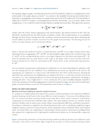
the topology adaptive graph convolutional network (TAGCN) method is defined as a multiplication of the
[37]
polynomials of the graph adjacency matrix . In contrast to the simplified formal spectral method that is
equivalent to propagating vertex features in a graph employed in the GCN method, the K-localized filter is
employed in TAGCN to explore crystal graph-structured data. Specifically, a set of receptive fields of size
ranging from 1 to K is defined to learn localized features on graph-structured data. This approach is given in

(6)

Finally, after the k-layer feature aggregation and transformation, the features learned by the GNN are
effectively transformed into the final density prediction results. This transformation is accomplished
through two linear layers, interspersed with a nonlinear activation function between them, enhancing the
model’s ability to predict complex outcomes from the graph-structured data. The learning process for
density of crystal structure can be expressed as follows:

(7)

(k)
where y denotes the predicted density of crystal structure, and H is the output feature matrix after
obtaining k-layers of aggregation. W and W are the learnable weight matrices for two linear layers, and
(1)
(2)
(0)
(1)
b and b are the corresponding bias vectors. According to Equation (6), the initial node features H = X,
(2)
where X represents the raw input features of the nodes in the graph. After k-layers, the final node-level
features learned by the GNN are represented as H , which serves as the transformed representation
(k)
(k)
X’= H .
For our method, hyperparameter optimization is conducted over 500 trials using Hyperopt optimizer, with
80% for training and 20% for validation. Final classification accuracies are reported on the test set. All
experiments are conducted on a Linux server with Nvidia RTX 4090 GPU (24GB memory). All methods
and GNN basic architectures are implemented according to PyTorch 2.1.2 and basic modules of PyTorch
Geometric 2.5.3. Key training parameters are fixed through hyperparameter optimization, including a
learning rate of lr ≈ 0.002, weight decay w ≈ 0.003, a batch size of 512, and 512 hidden channels. AdamW is
used as the optimizer, PowerMeanAggregation is selected for global pooling, and the model includes three
graph convolutional layers as learners. The detailed flow chart is shown in Figure 2.

RESULTS AND DISCUSSION
Machine learning modeling for specific crystal structures
To conduct an in-depth analysis and improve the accuracy of density prediction, this study first establishes
machine learning models based on the seven different crystal structures. This process of modeling utilizes
the five common machine learning models mentioned above. Each crystal structure’s intermetallic
compounds are extracted into individual data subsets. The input features selected are variables closely
related to density, such as atomic mass, atomic radius, electronegativity difference, and lattice parameters.
Six statistical treatments are applied to the elemental property data, such as calculating weighted averages,
weighted variances, geometric means, harmonic means, maximum values, minimum values, and weighted
sums. An initial feature set comprising 290 representative density features is generated, providing robust
data support for comprehensively exploring the multifactorial influences on intermetallic compound
density.

Figure 3 presents the performance of machine learning models in predicting density across different crystal
structures. A bar chart in the bottom right compares the accuracy of various machine learning models