Page 68 - Read Online

Page 374 Zhang et al. Intell Robot 2022;2(4):371­90 I http://dx.doi.org/10.20517/ir.2022.26

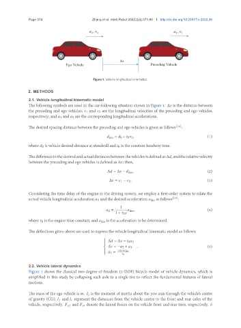
Figure 1. Vehicle longitudinal kinematics.

2. METHODS
2.1. Vehicle longitudinal kinematic model
The following symbols are used in the car-following situation shown in Figure 1: Δ is the distance between
the preceding and ego vehicles; 1 and 2 are the longitudinal velocities of the preceding and ego vehicles,
respectively; and 1 and 2 are the corresponding longitudinal accelerations.

The desired spacing distance between the preceding and ego vehicles is given as follows [28] :

des = 0 + 0 2 , (1)

where 0 is vehicle desired distance at standstill and 0 is the constant headway time.

Thedifferenceinthedesiredandactualdistancesbetweenthevehiclesisdefinedas Δ , andtherelativevelocity
between the preceding and ego vehicles is defined as Δ ; then,

Δ = Δ − des , (2)

Δ = 1 − 2 . (3)

Considering the time delay of the engine in the driving system, we employ a first-order system to relate the
actual vehicle longitudinal acceleration 2 and the desired acceleration des as follows [29] :

1
2 = des , (4)
1 + 0
where 0 is the engine time constant, and des is the acceleration to be determined.

The definitions given above are used to express the vehicle longitudinal kinematic model as follows:


 ¤
 Δ = Δ − 0 2
 
¤ . (5)
Δ = − 2 + 1
 − 2 + des
 ¤ 2 =

0

2.2. Vehicle lateral dynamics
Figure 2 shows the classical two-degree-of-freedom (2-DOF) bicycle model of vehicle dynamics, which is
simplified in this study by collapsing each axle to a single tire to reflect the fundamental features of lateral
motions.
The mass of the ego vehicle is . is the moment of inertia about the yaw axis through the vehicle’s centre
of gravity (CG). and represent the distances from the vehicle centre to the front and rear axles of the
vehicle, respectively. and denote the lateral forces on the vehicle front and rear tires, respectively.